
CHAPTER 10
Power Spectral Density
In the study of deterministic signals and systems, frequency domain techniques (e.g., Fourier transforms) provide a valuable tool that allows the engineer to gain significant insights into a variety of problems. In this chapter, we develop frequency domain tools for studying random processes. This will prepare us for the study of random processes in linear systems in the next chapter.
For a deterministic continuous signal, x(t), the Fourier transform is used to describe its spectral content. In this text, we write the Fourier transform as1
![]() (10.1)
(10.1)
and the corresponding inverse transform is
![]() (10.2)
(10.2)
For discrete-time signals, we could use a discrete Fourier transform or a z-transform. The Fourier transform, X(f), is referred to as the spectrum of x(t) since it describes the spectral contents of the signal. In general, X(f) is a complex function of frequency and hence we also speak of an amplitude (magnitude) spectrum, |X(f)|, and a phase spectrum, ∠X(f). In order to study random processes in the frequency domain, we seek a similar quantity which will describe the spectral characteristics of a random process.
The most obvious thing to do would be to try to define the Fourier transform of a random process as perhaps
![]() (10.3)
(10.3)
however, this leads to several problems. First of all, there are problems with existence. Since X(t) is a random process, there is not necessarily any guarantee that the integral exists for every possible realization, x(t). That is, not every realization of the random process may have a Fourier transform. Even for processes that are well-behaved in the sense that every realization has a well-defined Fourier transform, we are still left with the problem that X(f) is itself a random process. In Chapter 8, we described the temporal characteristics of random processes in terms of deterministic functions such as the mean function and the autocorrelation function. In a similar way, we seek a deterministic description of the spectral characteristics of a random process. The power spectral density (PSD) function, which is defined in the next section, will play that role.
10.1 Definition of PSD
To start with, for a random process X(t), define a truncated version of the random process as
 (10.4)
The energy of this random process is
 (10.5)
and hence the time-averaged power is
![]() (10.6)
(10.6)
The last equality is obtained using Parseval’s theorem. The quantity X to (f) is the Fourier transform of Xto (t). Since the random process has been truncated to a finite time interval, there will generally not be any problem with the existence of the Fourier transform. Note that P X to is a random variable and so to get the ensemble averaged power, we must take an expectation,
![]() (10.7)
(10.7)
The power in the (untruncated) random process X(t) is then found by passing to the limit as to → ∞,
 (10.8)
Define SXX (f) to be the integrand in Equation (10.8). That is, let
 (10.9)
Then, the average power in the process can be expressed as
![]() (10.10)
(10.10)
Therefore, this function of frequency which we have simply referred to as SXX (f) has the property that when integrated over all frequency, the total power in the process is obtained. In other words, SXX (f) has the units of power per unit frequency and so it is the power density function of the random process in the frequency domain. Hence, the quantity SXX (f) is given the name PSD. In summary, we have the following definition of PSD.
Definition 10.1: For a random process X(t), the power spectral density (PSD) is defined as
 (10.11)
where X to (f) is the Fourier transform of the truncated version of the process as described in Equation (10.4)
Several properties of the PSD function should be evident from Definition 10.1 and from the development that lead to that definition:
![]() (10.12a)
(10.12a)
![]() (10.12b)
(10.12b)
![]() (10.12c)
(10.12c)
![]() (10.12d)
(10.12d)
Example 10.1
As a simple example, consider a sinusoidal process X(t) = A sin(ωo t + Θ) with random amplitude and phase. Assume the phase is uniform over [0,2 π) and independent of the amplitude which we take to have an arbitrary distribution. Since each realization of this process is a sinusoid at frequency fo, we would expect that all of the power in this process should be located at f = fo (and f = −fo). Mathematically we have
![]()
where rect(t) is a square pulse of unit height and unit width and centered at t = 0. The Fourier transform of this truncated sinusoid works out to be
![]()
where the “sinc” function is sinc(x) = sin(πx)/(πx). We next calculate the expected value of the magnitude squared of this function.
![]()
The PSD function for this random process is then
![]()
To calculate this limit, we observe that as to gets large, the function g(f) = tosinc2(2fto) becomes increasingly narrower and taller. Thus, we could view the limit as an infinitely tall, infinitely narrow pulse. This is one way to define a delta function. One property of a delta function that is not necessarily shared by the function under consideration is that ![]() . Therefore, the limiting form of g(t) will have to be a scaled (in amplitude) delta function. To figure out what the scale factor needs to be, the integral of g(f) is calculated:
. Therefore, the limiting form of g(t) will have to be a scaled (in amplitude) delta function. To figure out what the scale factor needs to be, the integral of g(f) is calculated:
![]()
Therefore,
![]()
The resulting PSD is then simplified to
![]()
This is consistent with our intuition. The power in a sinusoid with amplitude A is A2/2. Thus, the average power in the sinusoidal process is E[A2]/2. This power is evenly split between the two points f= fo and f = −fo.
One important lesson to learn from the previous example is that even for very simplistic random processes, it can be quite complicated to evaluate the PSD using the definition given in Example 10.11. The next section presents a very important result that allows us to greatly simplify the process of finding the PSD of many random processes.
10.2 The Wiener–Khintchine–Einstein Theorem
Theorem 10.1 (Wiener–Khintchine–Einstein): For a wide sense stationary (WSS) random process X(t) whose autocorrelation function is given by RXX (τ), the PSD of the process is
![]() (10.13)
(10.13)
In other words, the autocorrelation function and PSD form a Fourier transform pair.
Proof: Starting from the definition of PSD,
 (10.14)
Using the assumption that the process is WSS, the autocorrelation function is only a function of a single time variable, t − s. Hence, the expression above is rewritten as
 (10.15)
It is noted that the preceding integrand is only a function of a single variable; therefore, with the appropriate change of variables, the double integral can be reduced to a single integral. The details are given in the following.
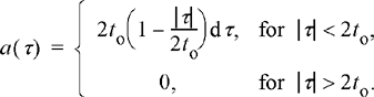
The region of integration is a square in the s-t plane of width 2to centered at the origin. Consider an infinitesimal strip bounded by the lines t − s = τ and t − s = τ + dτ. This strip is illustrated in Figure 10.1. Let a (τ) be the area of that strip which falls within the square region of integration. A little elementary geometry reveals that

Figure 10.1 Illustration of the change of variables for the double integral in Equation (10.15).
 (10.16)
To obtain the preceding result, one must neglect edge terms that contribute expressions which are quadratic in the infinitesimal dτ. Since the integrand in Equation (10.15) is a function only of t − s, it is constant (and equal to RXX (τ)e−j2πτ) over the entire strip. The double integral over the strip can therefore be written as the value of the integrand multiplied by the area of the strip. The double integral over the entire square can be written as a sum of the integrals over all the strips which intersect the square:
 (10.17)
Passing to the limit as dτ → 0, the sum becomes an integral resulting in
 (10.18)
The PSD function for the random process X(t) is then
 (10.19)
Passing to the limit as to → ∞ then gives the desired result in Equation (10.13).
While most of the random processes we deal with are WSS, for those that are not, Theorem 10.1 needs to be adjusted since the autocorrelation function for a non-stationary process would be a function of two time variables. For non-stationary processes, the Wiener–Khintchine–Einstein theorem is written as
![]() (10.20)
(10.20)
where in this case, 〈〉 represents a time average with respect to the time variable t. We leave it as an exercise to the reader to prove this more general version of the theorem.
Example 10.2
Let us revisit the random sinusoidal process, X(t) = A sin(ωo t + Θ), of Example 10.1. This time the PSD function will be calculated by first finding the autocorrelation function.
The autocorrelation function is only a function of τ and thus the PSD is simply the Fourier transform of the autocorrelation function,
![]()
This is exactly the same result that was obtained in Example 10.1 using the definition of PSD, but in this case, the result was obtained with much less work.
Example 10.3
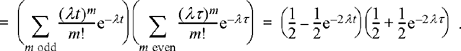
Now suppose we have a sinusoid with a random amplitude, but a fixed phase, X(t) = A sin(ωo t + θ). Here, the autocorrelation function is
![]()
![]()
In this case, the process is not WSS and so we must take a time average of the autocorrelation before we take the Fourier transform.

The time-averaged autocorrelation is exactly the same as the autocorrelation in the previous example, and hence, the PSD of the sinusoid with random amplitude and fixed phase is exactly the same as the PSD of the sinusoid with random amplitude and random phase.
Example 10.4
Next, consider a modified version of the random telegraph signal of Example 8.4. In this case, the process starts at X(0) = 1 and switches back and forth between X(t) = 1 and X(t) = −1, with the switching times being dictated by a Poisson point process with rate λ. A sample realization is shown in Figure 10.2. To find the PSD, we first find the autocorrelation function.

Figure 10.2 A sample realization for the random telegraph signal of Example 10.4.

The number of switches in a contiguous interval follows a Poisson distribution, and therefore

Since this is a function only of τ, we directly take the Fourier transform to find the PSD:
![]()
The autocorrelation function and PSD for this random telegraph signal are illustrated in Figure 10.3.
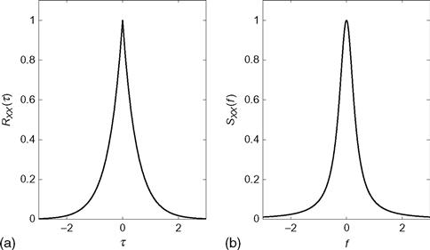
Figure 10.3 (a) Autocorrelation function and (b) PSD for the random telegraph signal of Example 10.4.
Example 10.5
To illustrate how some minor changes in a process can affect its autocorrelation and PSD, let us return to the random telegraph process as it was originally described in Example 8.4. As in the previous example, the process switches back and forth between two values as dictated by an underlying Poisson point process; however, now the two values of the process are X(t) ∈ {0,1} instead of X(t) ∈ {+1, − 1}. Also, the process starts at X(0) =0 instead of X(0) = 1. Noting that the product X(t)X(t + τ) is equal to zero unless both {X(t)=1} and {X(t + τ) = 1} are true, the autocorrelation function is calculated as
![]()
The last step was accomplished using some of the results obtained in Example 8.6 and assumes that τ is positive. If, on the other hand, τ is negative, then it turns out that
![]()
Clearly, this process is not stationary since the autocorrelation function is a function of both t and τ. Thus, before the Fourier transform is taken, the time average of the autocorrelation function must be computed.

In summary, the autocorrelation function can be concisely expressed as
![]()
The PSD function is then found to be
![]()
There are two differences between this result and that of Example 10.4. First, the total power (integral of PSD) in this process is 1/2 the total power in the process of the previous example. This is easy to see since when X(t) ∈ {0,1}, E[X2(t)] = 1/2, while when X(t) ∈ {+1, −1}, E[X2(t)] = 1. Second, in this example, there is a delta function in the PSD which was not present in the previous example. This is due to the fact that the mean of the process in this example was (asymptotically) equal to 1/2, whereas in the previous example it was zero. It is left as an exercise for the reader to determine if the initial conditions of the random process would have any effect on the PSD. That is, if the process started at X(0) = 1 and everything else remained the same, would the PSD change?
Definition 10.2: The cross spectral density between two random processes, X(t) and Y(t), is the Fourier transform of the cross correlation function:
![]() (10.21)
(10.21)
The cross spectral density does not have a physical interpretation nor does it share the same properties of the PSD function. For example, Sxy (f) is not necessarily real since Rxy (τ) is not necessarily even. The cross spectral density function does possess a form of symmetry known as Hermitian symmetry2,
![]() (10.22)
(10.22)
This property follows from the fact that RXY (τ) = Ryx (−τ). The proof of this property is left to the reader.
10.3 Bandwidth of a Random Process
Now that we have an analytical function which describes the spectral content of a signal, it is appropriate to talk about the bandwidth of a random process. As with deterministic signals, there are many definitions of bandwidth. Which definition is used depends on the application and sometimes on personal preference. Several definitions of bandwidth are given next. To understand these definitions, it is helpful to remember that when measuring the bandwidth of a signal (whether random or deterministic), only positive frequencies are measured. Also, we tend to classify signals according to where their spectral contents lies. Those signals for which most of the power is at or near direct current (d.c.) are referred to as lowpass signals, while those signals whose PSD is centered around some non-zero frequency, f = fo are referred to as bandpass processes.
Definition 10.3: For a lowpass process, the absolute bandwidth, Babs, is the largest frequency for which the PSD is non-zero. That is, Babs is the smallest value of B such that SXX (f) = 0 for all f > B. For a bandpass process, let BL be the largest value of B such that SXX (f) = 0 for all 0 ≤ f ≤ B and similarly let BR be the smallest value of B such that SXX (f) = 0 for all B ≤ f. Then Babs = BR − BL . In summary, the absolute bandwidth of a random process is the width of the band which contains all frequency components. The concept of absolute bandwidth is illustrated in Figure 10.4.

Figure 10.4 Measuring the absolute bandwidth of (a) a lowpass and (b) a bandpass process.
Definition 10.4: The 3 dB bandwidth (or half-power bandwidth), B3dB, is the width of the frequency band where the PSD is within 3 dB of its peak value everywhere within the band. Let Speak be the maximum value of the PSD. Then for a lowpass signal, B3dB is the largest value of B for which SXX (f) >Speak/2 for all frequencies such that 0 ≤f ≤ B. For a bandpass process, B3dB = Br−Bl, where SXX (f) >Speak/2 for all frequencies such that Bl ≤ f ≤ BR, and it is assumed that the peak value occurs within the band. The concept of 3 dB bandwidth is illustrated in Figure 10.5.

Figure 10.5 Measuring the 3 dB bandwidth of (a) a lowpass and (b) a bandpass process.
Definition 10.5: The root-mean-square (RMS) bandwidth, Brms, of a lowpass random process is given by
 (10.23)
This measure of bandwidth is analogous to using standard deviation as a measure of the width of a PDF. For bandpass processes, this definition is modified according to
 (10.24)
where
 (10.25)
It is left as an exercise to the reader to figure out why the factor of 4 appears in the preceding definition.
Example 10.6
Consider the random telegraph process of Example 10.4 where the PSD was found to be
![]()
The absolute bandwidth of this process is Babs = ∞. This can be seen from the picture of the PSD in Figure 10.2. To find the 3 dB bandwidth, it is noted that the peak of the PSD occurs at f =0 and has a value of Speak = λ−1. The 3 dB bandwidth is then the value of f for which Sxx (f) = 1/(2λ). This is easily found to be B3dB = λ/π. Finally, the RMS bandwidth of this process is infinite since
![]()
10.4 Spectral Estimation
The problem of estimating the PSD of a random process has been the topic of extensive research over the past several decades. Many books are dedicated to this topic alone and hence we cannot hope to give a complete treatment of the subject here; however, some fundamental concepts are introduced in this section that will provide the reader with a basic understanding of the problem and some rudimentary solutions. Spectral estimators are generally grouped into two classes, parametric and non-parametric. A parametric estimator assumes a certain model for the random process with several unknown parameters and then attempts to estimate the parameters. Given the model parameters, the PSD is then computed analytically from the model. On the other hand, a non-parametric estimator makes no assumptions about the nature of the random process and estimates the PSD directly. Since parametric estimators take advantage of some prior knowledge of the nature of the process, it would be expected that these estimators are more accurate. However, in some cases, prior knowledge may not be available, in which case a non-parametric estimator may be more appropriate. We start with a description of some basic techniques for non-parametric spectral estimation.
10.4.1 Non-parametric Spectral Estimation
Suppose we observe a random process, X(t), over some time interval (−to, to) (or a discrete-time process X[n] over some time interval [0, no− 1]) and we wish to estimate its PSD function. Two approaches immediately come to mind. The first method we will refer to as the direct method or the periodogram. It is based on the definition of PSD in Equation (10.11). The second method we will refer to as the indirect method or the correlation method. The basic idea here is to estimate the autocorrelation function and then take the Fourier transform of the estimated autocorrelation to form an estimate of the PSD. We first describe the correlation method. In all of the discussion on spectral estimation to follow, it is assumed that the random processes are WSS.
An estimate of the autocorrelation function of a continuous time random process can be formed by taking a time average of the particular realization observed:
 (10.26)
It is not difficult to show that this estimator is unbiased (i.e., E[![]() XX
(τ)] = RXX
(τ)), but at times, it is not a particularly good estimator, especially for large values of τ. The next example illustrates this fact.
XX
(τ)] = RXX
(τ)), but at times, it is not a particularly good estimator, especially for large values of τ. The next example illustrates this fact.
Example 10.7
Consider the random telegraph process of Example 10.4. A sample realization of this process is shown in Figure 10.6, along with the estimate of the autocorrelation function. For convenience, the true autocorrelation is shown as well. Note that the estimate matches quite well for small values of τ, but as |τ| → to, the estimate becomes very poor.

Figure 10.6 (a) A sample realization of the random telegraph signal and (b) the estimate of the autocorrelation function based on that realization. The dotted line is the true autocorrelation function.
In order to improve the quality of the autocorrelation estimate, it is common to introduce a windowing function to suppress the erratic behavior of the estimate at large values of τ. This is particularly important when estimating the PSD since the wild behavior at large values of |τ| will distort the estimate of the PSD at all frequencies once the Fourier transform of the autocorrelation estimate is taken.
Definition 10.6: For a WSS random process X(t), the windowed estimate of the autocorrelation function using a windowing function w (t) is given by
 (10.27)
There are many possible windowing functions that can be used. The previous autocorrelation estimate (without the windowing function) can be viewed as a windowed estimate with a rectangular window,
![]() (10.28)
(10.28)
Another option would be to use a triangular window,
 (10.29)
This would lead to the autocorrelation estimate,
 (10.30)
While this estimator is biased, the mean-squared error in the estimate will generally be smaller than when the rectangular window is used. Much of the classical spectral estimation theory focuses on how to choose an appropriate window function to satisfy various criteria.
Example 10.8
The autocorrelation function of the random telegraph signal is once again estimated, this time with the windowed autocorrelation estimator using the triangular window. The sample realization as well as the autocorrelation estimate are shown in Figure 10.7. Note this time that the behavior of the estimate for large values of τ is more controlled.

Figure 10.7 (a) A sample realization of the random telegraph signal and (b) the windowed estimate of the autocorrelation function (using a triangular window) based on that realization.
Once an estimate of the autocorrelation can be found, the estimate of the PSD is obtained through Fourier transformation.
Definition 10.7: For a WSS random process X(t), the correlation-based estimate (with windowing function w (t)) of the PSD is given by
 (10.31)
Example 10.9
The PSD estimates corresponding to the autocorrelation estimates of the previous example are illustrated in Figure 10.8. There the correlation-based PSD estimates are plotted and compared with the true PSD. Note that when no windowing is used, the PSD estimate tends to overestimate the true PSD. Another observation is that it appears from these results that the PSD estimates could be improved by smoothing. We will elaborate on that shortly.

Figure 10.8 (a) A sample realization of the random telegraph signal and (b, c) the estimate of the PSD function. Plot (b) is for the unwindowed estimator while the plot (c) is for the triangular windowed estimator. For both PSD plots, the smooth thick line is the true PSD.
The next approach we consider for estimating the PSD of a random process is to directly use the definition of PSD in Equation (10.11). This approach is referred to as the periodogram estimate.
Definition 10.8: Given an observation of the process X(t) over an interval (−to, to), X to (t), the periodogram estimate of the PSD is
![]() (10.32)
(10.32)
Theorem 10.2: The periodogram estimate of the PSD is equivalent to the autocorrelation-based estimate with a triangular window. That is,
![]() (10.33)
(10.33)
Proof: The proof of this theorem is a fairly elementary exercise in manipulating the properties of Fourier transforms. Recall that for any two signals, x (t) and y (t), the product of their spectra form a transform pair with the convolution of the two signals. That is, f[x (t) * y (t)] = X(f) Y(f). Applying this to Equation (10.32) results in
 (10.34)
An example of the periodogram was given in Figure 10.8c. At the time, it was referred to as the correlation-based estimate with a triangular windowing function. Now, it is clear that the two are the same. It was mentioned in Example 10.9, that the quality of the periodogram might be improved by smoothing the PSD estimate. This can be accomplished by convolving ![]() (p)
XX
(f) with some smoothing function,
(p)
XX
(f) with some smoothing function, ![]() (f).
(f).
Definition 10.9: The smoothed periodogram with smoothing function ![]() (f) is given by
(f) is given by
![]() (10.35)
(10.35)
The smoothed periodogram can be viewed in terms of the correlation-based estimate as well. Note that if ![]() , then
, then
![]() (10.36)
(10.36)
Therefore, the smoothed periodogram is nothing more than the windowed correlation-based estimate with a window that is the product of w (t) and the triangular window. This seems to indicate that there would be some potential benefit to using windowing functions other than what has been presented here. The reader is referred to the many books on spectral estimation for discussions of other possibilities.
In all of the spectral estimators presented thus far, an ensemble average was estimated using a single realization. A better estimate could be obtained if several independent realizations of the random process were observed and a sample average were used to replace the ensemble average. Even though we may be able to observe only a single realization, it may still be possible to achieve the same effect. This is done by breaking the observed time waveform into segments and treating each segment as an independent realization of the random process. The periodogram is computed on each segment and then the resulting estimates are averaged.
Example 10.10
 Figure 10.9 compares the periodogram estimate of the PSD of the random telegraph signal with and without segmentation. In plot (b), no segmentation is used, while in plot (c), the data are segmented into M =8 frames. A periodogram is computed for each frame and the results are then averaged. Note the improvement in the PSD estimate when the segmentation is used. Also note that there is a slight bias appearing in the segmented estimate. This is most noticeable at the higher frequencies. This bias will get worse as more segments are used. There is a trade-off in wanting to use a large value of M to reduce the “jitter” in the estimate and wanting to use a small value of M to keep the bias to a minimum. The following MATLAB functions were used to implement the periodogram estimates with and without segmentation. This same functions can be used to estimate the PSD of any input signal.

Figure 10.9 (a) A sample realization of the random telegraph signal and (b,c) the periodogram estimate of the PSD function. Plot (b) is for the unsegmented data while plot (c) is for when the data are segmented into M =8 frames. For both PSD plots, the smooth thick line is the true PSD.


10.4.2 Parametric Spectral Estimation
In parametric spectral estimation, a general model of the data is assumed, which usually contains one or more unknown parameters. Given the general model, the PSD can be calculated analytically. The problem then becomes one of estimating the unknown parameters and plugging the result into the analytic form of the PSD. To provide an example of how this general approach works, we present a specific class of random process models.
Definition 10.10: Given a process X[n] with known statistics, a new process, Y[n], is formed according to the difference equation
![]() (10.37)
(10.37)
This process is referred to as an autoregressive moving average process (ARMA). As special cases, if all of the ai are equal to zero (except a0, which is usually set equal to unity), then Equation (10.37) simplifies to
![]() (10.38)
(10.38)
and the process is referred to as a moving average (MA) process. The notation MA(q) is used to refer to a qth order MA process. If all of the bi are equal to zero except for b0, then the difference equation becomes
![]() (10.39)
(10.39)
and the process is referred to as an autoregressive (AR) process. The notation AR(p) is used to refer to a pth order AR process. For the general case, the notation ARMA(p,q) is used.
To demonstrate the basic principles of parametric estimation, suppose it was determined that a certain random process, Y[n], is well modeled by an AR(1) model,
![]() (10.40)
(10.40)
where X[n] is an IID random process with zero-mean and a variance of σ2 X . It is noted that
![]() (10.41)
(10.41)
![]() (10.42)
(10.42)
![]() (10.43)
(10.43)
 (10.44)
Using this expression, the autocorrelation function of the AR(1) process can be computed.
 (10.45)
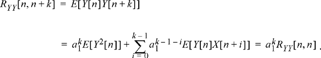
The last step is accomplished using the fact that Y[n] is independent of X[n + i] for i > 0. The expression RYY [n, n] is calculated according to
![]() (10.46)
(10.46)
Assuming that the process Y[n] is WSS3, this recursion becomes
 (10.47)
Therefore, the autocorrelation function of the AR(1) process is
 (10.48)
Assuming that the samples of this discrete-time process are taken at a sampling interval of Δt, the PSD of this process works out to be
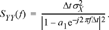 (10.49)
For this simple AR(1) model, the PSD can be expressed as a function of two unknown parameters, a1 and σ2 X . The problem of estimating the PSD then becomes one of estimating the two parameters and then plugging the result into the general expression for the PSD. In many cases, the total power in the process may be known, which eliminates the need to estimate σ2 X . Even if that is not the case, the value of σ2 X is just a multiplicative factor in the expression for PSD and does not change the shape of the curve. Hence, in the following, we focus attention on estimating the parameter, a1.
Since we know the AR(1) model satisfies the recursion of Equation (10.40), the next value of the process can be predicted from the current value according to
![]() (10.50)
(10.50)
This is known as linear prediction since the predictor of the next value is a linear function of the current value. The error in this estimate is
![]() (10.51)
(10.51)
Typically, we choose as an estimate of a1 the value of ![]() 1 that makes the linear predictor as good as possible. Usually, “good” is interpreted as minimizing the mean-square error, which is given by
1 that makes the linear predictor as good as possible. Usually, “good” is interpreted as minimizing the mean-square error, which is given by
![]() (10.52)
(10.52)
Differentiating the mean-square error with respect to ![]() 1 and setting equal to zero results in
1 and setting equal to zero results in
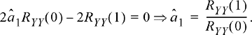 (10.53)
Of course, we do not know what the autocorrelation function is. If we did, we would not need to estimate the PSD. So, the preceding ensemble averages must be replaced with sample averages, and the minimum mean-square error (MMSE) linear prediction coefficient is given by
 (10.54)
Note that we have used a lower case y [n] in Equation (10.54) since we are dealing with a single realization rather than the ensemble Y[n].
Example 10.11
In this example, we use the AR(1) model to estimate the PSD of the random telegraph process. Clearly, the AR(1) model does not describe the random telegraph process; however, the autocorrelation function of the random telegraph signal is a two-sided exponential, as is the autocorrelation function of the AR(1) process. As a consequence, we expect this model to give good results. The results are shown in Figure 10.10. Notice how nicely the estimated PSD matches the actual PSD.

Figure 10.10 (a) A sample realization of the random telegraph signal and (b) the parametric estimate of the PSD function based on the AR(1) model.
In the previous example, the results were quite good because the functional form of the PSD of the AR(1) process nicely matched the functional form of the true PSD. If the fit had not been so good, it might have been necessary to move to a higher order AR(p) model. In the exercises at the end of the chapter (see Exercises 10.19 and 10.20), the reader is led through the problem of finding the MMSE linear prediction coefficients for a general AR(p) model. The problem of analytically finding the PSD of the AR(p) process is dealt with in the next chapter (also see Exercise 10.18).
10.5 Thermal Noise
The most commonly encountered source of noise in electronic systems is that caused by thermal agitation of electrons in any conductive material, which is commonly referred to as thermal noise. Unlike shot noise, thermal noise does not require the presence of a direct current and hence is always present. We will not delve into the underlying thermodynamics to derive a model for this type of noise, but rather will just summarize some of the important results. Nyquist’s theorem states that for a resistive element with an impedance of r ohms, at a temperature of tk (measured in Kelvin), the mean-square voltage of the thermal noise measured in a incremental frequency band of width Δf centered at frequency f is found to be
 (10.55)
where
Typically, a practical resistor is modeled as a Thevenin equivalent circuit, as illustrated in Figure 10.11, consisting of a noiseless resistor in series with a noise source with a mean-square value as specified in the previous equation. If this noisy resistor was connected to a resistive load of impedance rL, the average power delivered to the load would be

Figure 10.11 A Thevenin equivalent circuit for a noisy resistor.
 (10.56)
The power delivered to the load is maximized when the source and the load impedance are matched (i.e., rL = r). It is common to refer to the maximum power that can be delivered to a load as the available power. For a noisy resistor, the available power (in a bandwidth of Δf) is
 (10.57)
The PSD of the thermal noise in the resistor is then
 (10.58)
The extra factor of 1/2 is due to the fact that our PSD function is a two-sided function of frequency, and so the actual power in a given frequency band is evenly split between the positive and negative frequencies. Note that the power available to a load and the resulting PSD are independent of the impedance of the resistor, r.
This PSD function is plotted in Figure 10.12 for several different temperatures. Note that for frequencies that are of interest in most applications (except optical, infrared, etc.), the PSD function is essentially constant. It is straightforward (and left as an exercise to the reader) to show that this constant is given by

Figure 10.12 PSD of thermal noise in a resistor.
![]() (10.59)
(10.59)
where we have defined the constant No = kt f . At tk = 298°K 4, the parameter No takes on a value of = 4.11×10⁻²¹W/Hz = − 173.86 dBm/Hz.
It is common to use this simpler function as a model for the PSD of thermal noise. Because the PSD contains equal power at all frequencies, this noise model is referred to as white noise (analogous to white light, which contains all frequencies). The corresponding autocorrelation function is
![]() (10.60)
(10.60)
It should be pointed out that the noise model of Equation (10.59) is a mathematical approximation to the actual PSD. There is no such thing as truly white noise, since such a process (if it existed) would have infinite power and would destroy any device we tried to measure it with. However, this mathematical model is simple, easy to work with, and serves as a good approximation to thermal noise for most applications.
In addition to modeling thermal noise as having a flat PSD, it can also be shown that the first-order characteristics of thermal noise can be well approximated with a zero-mean Gaussian process. We say that thermal noise is zero-mean white Gaussian noise (WGN) with a (two-sided) PSD of No/2. While thermal noise is the most common source of noise in electronic devices, there are other sources as well. Shot noise was discussed at the end of Chapter 8. In addition, one may encounter flicker noise, which occurs primarily in active devices; burst or popcorn noise, which is found in integrated circuits and some discrete transistors; avalanche noise, which is produced by avalanche breakdown in a p–n junction; as well as several other types of noise. For the purposes of this text, we will stick with the white Gaussian model of thermal noise.
10.6 Engineering Application: PSDs of Digital Modulation Formats
In this section, we evaluate the PSD of a class of signals that might be used in a digital communication system. Suppose we have a sequence of data symbols {Bk } that we wish to convey across some communication medium. We can use the data symbols to determine the amplitude of a sequence of pulses which we would then transmit across the medium (e.g., a twisted copper pair, or an optical fiber). This is know as pulse amplitude modulation (PAM). If the pulse amplitudes are represented by the sequence of random variables {…, A−2, A−1, A0, A1, A2, …} and the basic pulse shape is given by the waveform p(t), then the transmitted signal might be of the form
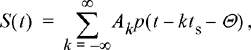 (10.61)
where ts is the symbol interval (that is, one pulse is launched every ts seconds) and Θ is a random delay, which we take to be uniformly distributed over [0, ts) and independent of the pulse amplitudes. The addition of the random delay in the model makes the process S(t) WSS. This is not necessary and the result we will obtain would not change if we did not add this delay, but it does simplify slightly the derivation.
If the data symbols are drawn from an alphabet of size 2n symbols, then each symbol can be represented by an n-bit word, and thus the data rate of the digital communication system is r = n/ts bits/second. The random process S(t) used to represent this data has a certain spectral content, and thus requires a communications channel with a bandwidth adequate to carry that spectral content. It would be interesting to see how the required bandwidth relates to the data rate. Toward that end, we seek to determine the PSD of the PAM signal S(t). We will find the PSD by first computing the autocorrelation function of S(t) and then converting this to PSD via the Wiener–Khintchine–Einstein Theorem.
Using the definition of autocorrelation, the autocorrelation function of the PAM signal is given by
 (10.62)
To simplify notation, we define RAA [n] to be the autocorrelation function of the sequence of pulse amplitudes. Note that we are assuming the sequence is stationary (at least in the wide sense). Going through a simple change of variables (v = t − kts − θ) then results in
 (10.63)
Finally, we go through one last change of variables (n = m − k) to produce
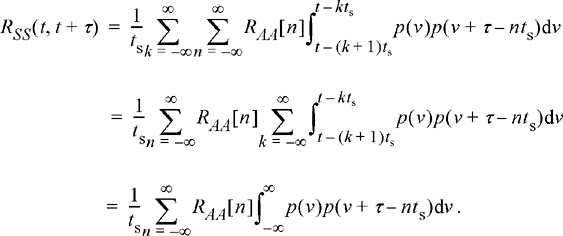 (10.64)
To aid in taking the Fourier transform of this expression, we note that the integral in the previous equation can be written as a convolution of p(t) with p(−t),
![]() (10.65)
(10.65)
Using the fact that convolution in the time domain becomes multiplication in the frequency domain along with the time reversal and time shifting properties of Fourier transforms (see Appendix C), the transform of this convolution works out to be
 (10.66)
where P (f) = f[p(t)] is the Fourier transform of the pulse shape used. With this result, the PSD of the PAM signal is found by taking the transform of Equation (10.64), resulting in
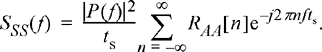 (10.67)
It is seen from the previous equation that the PSD of a PAM signal is the product of two terms, the first of which is the magnitude squared of the pulse shape’s spectrum, while the second term is essentially the PSD of the discrete sequence of amplitudes. As a result, we can control the spectral content of our PAM signal by carefully designing a pulse shape with a compact spectrum and also by introducing memory into the sequence of pulse amplitudes.
Example 10.12
To start with, suppose the pulse amplitudes are an IID sequence of random variables which are equally likely to be +1 or − 1. In that case, RAA [n] = δ[n] and the PSD of the sequence of amplitudes is
![]()
In this case, SSS (f) = |P(f)|2/ts and the spectral shape of the PAM signal is completely determined by the spectral content of the pulse shape. Suppose we use as a pulse shape a square pulse of height a and width ts,
![]()
The PSD of the resulting PAM signal is then SSS (f) = a2 tssinc2(fts). Note that the factor a2 ts is the energy in each pulse sent, Ep. A sample realization of this PAM process along with a plot of the PSD is given in Figure 10.13. Most of the power in the process is contained in the main lobe, which has a bandwidth of 1/ts (equal to the data rate), but there is also a non-trivial amount of power in the sidelobes, which die off very slowly. This high-frequency content can be attributed to the instantaneous jumps in the process. These frequency sidelobes can be suppressed by using a pulse with a smoother shape. Suppose, for example, we used a pulse which was a half-cycle of a sinusoid of height a,

Figure 10.13 (a) A sample realization and (b) the PSD of a PAM signal with square pulses.

The resulting PSD of the PAM signal with half-sinusoidal pulse shapes is then

In this case, the energy in each pulse is Ep = a2 ts/2. As shown in Figure 10.14, the main lobe is now 50 % wider than it was with square pulses, but the sidelobes decay much more rapidly.

Figure 10.14 (a) A sample realization and (b) the PSD of a PAM signal with half-sinusoidal pulses.
Example 10.13
In this example, we show how the spectrum of the PAM signal can also be manipulated by adding memory to the sequence of pulse amplitudes. Suppose the data to be transmitted {…, B−2, B−1, B0, B1, B2, …} is an IID sequence of Bernoulli random variables, Bk ∈ {+1, −1}. In the previous example, we formed the pulse amplitudes according to Ak = Bk . Suppose instead we formed these amplitudes according to Ak = Bk + B k−1. Now the pulse amplitudes can take on three values (even though each pulse still only carries one bit of information). This is known as duobinary precoding. The resulting autocorrelation function for the sequence of pulse amplitudes is

The PSD of this sequence of pulse amplitudes is then
![]()
This expression then multiplies whatever spectral shape results from the pulse shape chosen. The PSD of duobinary PAM with square pulses is illustrated in Figure 10.15. In this case, the duobinary precoding has the benefit of suppressing the frequency sidelobes without broadening the main lobe.

Figure 10.15 (a) A sample realization and (b) the PSD of a PAM signal with duobinary precoding and square pulses.
Example 10.14
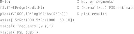
The following MATLAB code creates a realization of a binary PAM signal where the pulse amplitudes are either +1 or − 1. In this example, a half-sinusoidal pulse shape is used, but the code is written so that it is easy to change the pulse shape (just change the 6th line where the pulse shape is assigned to the variable p). After a realization of the PAM signal is created, the PSD of the resulting signal is estimated using the segmented periodogram technique given in Example 10.10. The resulting PSD estimate is shown in Figure 10.16. Note the agreement between the estimate and the actual PSD shown in Figure 10.14. The reader is encouraged to try running this program with different pulse shapes to see how the pulse shape changes the spectrum of the PAM signal.

Figure 10.16 An estimate of the PSD of a PAM signal with half-sinusoidal pulse shapes.

Exercises
Section 10.1: Definition of PSD
10.1 Find the PSD of the process described in Exercise 8.1.
10.2 Find the PSD of the process described in Exercise 8.2.
10.3 Consider a constant random process, X(t) = A, where A is a random variable. Use Definition 10.1 to calculate the PSD of X(t).
Section 10.2: Wiener–Khintchine–Einstein Theorem
10.4 Consider a random process of the form
![]()
where b is a constant, Θ is a uniform random variable over [0, 2π), and Ψ is a random variable which is independent of Θ and has a PDF, fΨ(ψ). Find the PSD, SXX (f) in terms of fΨ(ψ). In so doing, prove that for any S(f) which is a valid PSD function, we can always construct a random process with PSD equal to S(f).
10.5 Let X(t) = A cos (ωt) + B sin (ωt) where A and B are independent, zero-mean, identically distributed, non-Gaussian random variables.
(a) Show that X(t) is WSS, but not strict sense stationary. Hint: For the latter case consider E[X3 (t)]. Note: If A and B are Gaussian, then X(t) is also stationary in the strict sense.
10.6 Let ![]() ) where all of the ω
n
are non-zero constants, the an
are constants, and the θ
n
are IID random variables, each uniformly distributed over [0, 2 π).
) where all of the ω
n
are non-zero constants, the an
are constants, and the θ
n
are IID random variables, each uniformly distributed over [0, 2 π).
10.7 Let ![]() be a random process, where An
and Bn
are random variables such that E[An
] = E[Bn
] = 0, E[AnBm
] = 0, E[AnAm
] = δ
n,m
E[A2
n
], and E[BnBm
] = δ
n,m
E[B2
n
] for all m and n, where δ
n,m
is the Kronecker delta function. This process is sometimes used as a model for random noise.
be a random process, where An
and Bn
are random variables such that E[An
] = E[Bn
] = 0, E[AnBm
] = 0, E[AnAm
] = δ
n,m
E[A2
n
], and E[BnBm
] = δ
n,m
E[B2
n
] for all m and n, where δ
n,m
is the Kronecker delta function. This process is sometimes used as a model for random noise.
(a) Find the time-varying autocorrelation function Rxx (t, t + τ).
10.8 Find the PSD for a process for which RXX (τ) = 1 for all τ.
10.9 Suppose X(t) is a stationary zero-mean Gaussian random process with PSD, Sxx (f).
10.10 Consider a random sinusoidal process of the form X(t) = b cos (2πft + Θ), where Θ has an arbitrary PDF, fΘ(θ). Analytically determine how the PSD of X(t) depends on fΘ(θ). Give an intuitive explanation for your result.
10.11 Let s(t) be a deterministic periodic waveform with period to. A random process is constructed according to X(t) = s (t − T) where T is a random variable uniformly distributed over [0, to). Show that the random process X(t) has a line spectrum and write the PSD of X(t) in terms of the Fourier Series coefficients of the periodic signal s(t).
10.12 A sinusoidal signal of the form X(t) = bcos(2πfo
t + Θ) is transmitted from a fixed platform. The signal is received by an antenna which is on a mobile platform that is in motion relative to the transmitter, with a velocity of V relative to the direction of signal propagation between the transmitter and receiver. Therefore, the received signal experiences a Doppler shift and (ignoring noise in the receiver) is of the form
![]()
where c is the speed of light. Find the PSD of the received signal if V is uniformly distributed over (−vo, vo). Qualitatively, what does the Doppler effect do to the PSD of the sinusoidal signal?
10.13 Two zero-mean discrete random processes, X[n] and Y[n], are statistically independent and have autocorrelation functions given by RXX [k] = (1/2)k and RYY [k] = (1/3)k. Let a new random process be Z[n] = X[n] + Y[n].
(a) Find RZZ [k]. Plot all three autocorrelation functions.
(b) Determine all three PSD functions analytically and plot the PSDs.
10.14 Let Sxx (f) be the PSD function of a WSS discrete-time process X[n]. Recall that one way to obtain this PSD function is to compute RXX [n] = E[X[k]X[k + n]] and then take the DFT of the resulting autocorrelation function. Determine how to find the average power in a discrete-time random process directly from the PSD function, SXX (f).
10.15 A binary phase shift keying signal is defined according to
![]()
for all n, and B[n] is a discrete-time Bernoulli random process that has values of+1 or −1.
10.16 Let X(t) be a random process whose PSD is shown in the accompanying figure. A new process is formed by multiplying X(t) by a carrier to produce
![]()
where Θ is uniform over [0, 2π) and independent of X(t). Find and sketch the PSD of the process Y(t).

Section 10.3: Bandwidth of a Random Process
10.18 Develop a formula to compute the RMS bandwidth of a random process, X(t), directly from its autocorrelation function, RXX (τ).
10.19 A random process has a PSD function given by

(a) Find the absolute bandwidth.
(c) Find the RMS bandwidth.
Can you generalize your result to a spectrum of the form
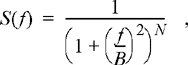
where N is an integer greater than 1?
10.20 A random process has a PSD function given by


Section 10.4: Spectral Estimation
10.21 Consider the linear prediction random process X[n] = (1/2)X[n − 1] + E[n], n = 1, 2, 3, …, where X[0] = 0 and E[n] is a zero-mean, IID random process.
10.22 Consider an AR(2) process which is described by the recursion
![]()
where X[n] is an IID random process with zero-mean and variance σ2 X .
(a) Show that the autocorrelation function of the AR(2) process satisfies the difference equation,
![]()
(b) Show that the first two terms in the autocorrelation function satisfy

From these two equations, solve for RYY[0] and RYY[1] in terms of a1, a2, and σ2X
(c) Using the difference equation in part (a) together with the initial conditions in part (b), find a general expression for the autocorrelation function of an AR(2) process.
(d) Use your result in part (c) to find the PSD of an AR(2) process.
10.23 Suppose we use an AR(2) model to predict the next value of a random process based on observations of the two most recent samples. That is, we form
![]()
(a) Derive an expression for the mean-square estimation error,
![]()
(b) Find the values of the prediction coefficients, a1 and a2, that minimize the mean-square error.
10.24 Extend the results of Exercise 10.23 to a general AR(p) model. That is, suppose we wish to predict the next value of a random process by forming a linear combination of the p most recent samples:

Find an expression for the values of the prediction coefficients which minimize the mean-square prediction error.
10.25 Show that the estimator for the autocorrelation function, ![]() XX(τ), described in Equation (10.26) is unbiased. That is, show that E[
XX(τ), described in Equation (10.26) is unbiased. That is, show that E[![]() XX(τ)] = RXX(τ).
XX(τ)] = RXX(τ).
10.26 Suppose X(t) is a zero-mean, WSS, Gaussian random process. Find an expression for the variance of the estimate of the autocorrelation function, ![]() XX(τ), given in Equation (10.26). That is, find Var(
XX(τ), given in Equation (10.26). That is, find Var(![]() XX(τ). Hint: Remember
XX(τ). Hint: Remember ![]() xx(i) is unbiased (see Exercise 10.25) and you might find the Gaussian moment factoring theorem (see Exercise 6.18) useful.
xx(i) is unbiased (see Exercise 10.25) and you might find the Gaussian moment factoring theorem (see Exercise 6.18) useful.
10.27 Using the expression for Var(![]() XX(τ)) found in Exercise 10.26, show that as |τ|→2to, Var(
XX(τ)) found in Exercise 10.26, show that as |τ|→2to, Var(![]() XX(τ))> Var(X(t)) and therefore, the estimate of the autocorrelation function is at least as noisy as the process itself as |τ|→2to.
XX(τ))> Var(X(t)) and therefore, the estimate of the autocorrelation function is at least as noisy as the process itself as |τ|→2to.
10.28 Determine whether or not the periodogram is an unbiased estimate of the PSD.
10.29 Suppose we form a smoothed periodogram of the PSD, ![]() (wp)XX(f), as defined in Equation (10.35), using a rectangular smoothing function,
(wp)XX(f), as defined in Equation (10.35), using a rectangular smoothing function,
![]()
where fΔ is the width of the rectangle. If we want to form the same estimator using a windowed correlation-based estimate, what window function (in the time domain) should we use?
Section 10.5: Thermal Noise
(a) Prove that the expression for the PSD of thermal noise in a resistor converges to the constant No/2 = ktk/2 as f → 0.
(b) Assuming a temperature of 298 °K, find the range of frequencies over which thermal noise has a PSD which is within 99% of its value at f = 0.
(c) Suppose we had a very sensitive piece of equipment which was able to accurately measure the thermal noise across a resistive element. Furthermore, suppose our equipment could respond to a range of frequencies which spanned 50 MHz. Find the power (in watts) and the RMS voltage (in volts) that we would measure across a 75 Ω resistor. Assume the equipment had a load impedance matched to the resistor.
10.31 Suppose two resistors of impedance r1 and r2 are placed in series and held at different physical temperatures, t1 and t2. We would like to model this series combination of noisy resistors as a single noiseless resistor with an impedance of r = r1 + r2, together with a noise source with an effective temperature of te. In short, we want the two models shown in the accompanying figure to be equivalent. Assuming the noise produced by the two resistors is independent, what should te
, the effective noise temperature of the series combination of resistors, be? If the two resistors are held at the same physical temperature, is the effective temperature equal to the true common temperature of the resistors?

10.32 Repeat Exercise 10.31 for a parallel combination of resistors.
MATLAB Exercises
(a) Create a random process X[n] where each sample of the random process is an IID, Bernoulli random variable equally likely to be ±1. Form a new process according to the MA(2) model ![]() . Assume X[n] = 0 for n ≤ 0.
. Assume X[n] = 0 for n ≤ 0.
(b) Compute the time-average autocorrelation function 〈Y[n] Y[n + k]〉 from a single realization of this process.
(c) Compute the ensemble average autocorrelation function E[Y[n]Y[n + k]] from several realizations of this process. Does the process appear to be ergodic in the autocorrelation?
(d) Estimate the PSD of this process using the periodogram method.
(a) Create a random process X[n] where each sample of the random process is an IID, Bernoulli random variable equally likely to be ±1. Form a new process according to the AR(2) model ![]() . Assume Y[n] = 0 for n ≤ 0.
. Assume Y[n] = 0 for n ≤ 0.
(b) Compute the time-average autocorrelation function 〈Y[n]Y[n + k]〉 from a single realization of this process.
(c) Compute the ensemble average autocorrelation function E[Y[n] Y[n + k]] from several realizations of this process. Does the process appear to be ergodic in the autocorrelation?
(d) Estimate the PSD of this process using the periodogram method.
(a) For the process in Exercise 10.34, find a parametric estimate of the PSD by using an AR(1) model. Compare the resulting PSD estimate with the non-parametric estimate found in Exercise 10.34(d). Explain any differences you see.
(b) Again, referring to the process in Exercise 10.34, find a parametric estimate of the PSD this time using an AR(2) model. Compare the resulting PSD estimate with the non-parametric estimate found in Exercise 10.34(d). Explain any differences you see.
(a) Write a MATLAB program to create a realization of a binary PAM signal with square pulses. You can accomplish this with a simple modification to the program given in Example 10.14. Call this signal x(t).
(b) We can create a frequency shift keying (FSK) signal according to
![]()
where ts is the duration of the square pulses in x(t) and fc is the carrier frequency. Write a MATLAB program to create a 10 ms realization of this FSK signal assuming ts = 100 μs and fc = 20 kHz.
(c) Using the segmented periodogram, estimate the PSD of the FSK signal you created in part (b).
(d) Estimate the 30 dB bandwidth of the FSK signal. That is, find the bandwidth where the PSD is down 30 dB from its peak value.
10.37 Construct a signal plus noise random sequence using 10 samples of the following:
![]()
where N[n] is a sequence of zero-mean, unit variance, IID Gaussian random variables, f0 = 0.1/ts = 100 kHz, and ts = 1μs is the time between samples of the process.
(a) Calculate the periodogram estimate of the PSD, Sxx(f).
(b) Calculate a parametric estimate of the PSD using AR models with p = 1, 2, 3, and 5. Compare the parametric estimates with the periodogram. In your opinion, which order AR model is the best fit.
(c) Repeat parts (a) and (b) using 100 samples instead of 10.
10.38 Construct a signal plus noise random sequence using 10 samples of:
![]()
where N[n] is a sequence of zero-mean, unit variance, IID Gaussian random variables, and f1 = 0.1/ts = 100 kHz, f2 = 0.4/ts = 400 kHz, and ts = 1μs is the time between samples of the process.
(a) Calculate the periodogram estimate of the PSD, Sxx(f).
(b) Calculate a parametric estimate of the PSD using AR models with p = 3, 4, 5, 6, and 7. Compare the parametric estimates with the periodogram. In your opinion, which order AR model is the best fit.
(c) Repeat parts (a) and (b) using 100 samples instead of 10.
1 Even though we use an upper case letter to represent a Fourier transform, it is not necessarily random. Clearly, the Fourier transform of a non-random signal is also not random. While this is inconsistent with our previous notation of using upper case letters to represent random quantities, this notation of using upper case letters to represent Fourier Transforms is so common in the literature, we felt it necessary to retain this convention. The context should make it clear whether a function of frequency is random or not.
2 Here and throughout the text, the superscript * refers to the complex conjugate.
3 It will be shown in the next chapter that this is the case provided that X[n] is WSS.
4 Most texts use tk = 290 °K as “room temperature”; however, this corresponds to a fairly chilly room (17°C ≈ 63°F). On the other hand, tk = 298°K is a more balmy (25°C ≈ 77°F) environment. These differences would only change the value of No by a small fraction of a dB.