
CHAPTER 3
Random Variables, Distributions, and Density Functions
At the end of the last chapter, we introduced the concept of a random variable and gave several examples of common discrete random variables. These random variables were described by their probability mass functions. While this description works fine for discrete random variables, it is inadequate to describe random variables that take on a continuum of values. We will illustrate this through an example shortly. In this chapter, we introduce the cumulative distribution function (CDF) as an alternative description of random variables that is appropriate for describing continuous as well as discrete random variables. A related function, the probability density function (PDF), is also covered. With these tools in hand, the concepts of random variables can be fully developed. Several examples of commonly used continuous random variables are also discussed in this chapter.
To show the need for an alternative to the probability mass function, consider a discrete random variable, X, that takes on values from the set {0, 1/N, 2/N, …, (N – 1)/N} with equal probability. That is, the probability mass function of X is
![]() (3.1)
(3.1)
This is the type of random variable that is produced by “random” number generators in high level languages such as Fortran and C, as well as math packages such as MATLAB, MathCAD, and Mathematica. In these cases, N is taken to be a fairly large number so that it appears that the random number can be anything in the continuous range [0, 1). The reader is referred to Chapter 12, for more details on how computer-generated random numbers work. For now, consider the limiting case as N → ∞ so that the random variable can truly fall anywhere in the interval [0, 1). One curious result of passing to the limit is that now
![]() (3.2)
(3.2)
That is, each point has zero probability of occurring. Yet, something has to occur! This problem is common to continuous random variables, and it is clear that the probability mass function is not a suitable description for such a random variable. The next sections develop two alternative descriptions for continuous random variables, which will be used extensively throughout the rest of the text.
3.1 The Cumulative Distribution Function
Since a continuous random variable will typically have a zero probability of taking on a specific value, we avoid talking about such probabilities. Instead, events of the form {X ≤ x} can be considered.
Definition 3.1: The CDF of a random variable, X, is
![]() (3.3)
(3.3)
From this definition, several properties of the CDF can be inferred. First, since the CDF is a probability, it must take on values between 0 and 1. Since random variables are real valued, it is easy to conclude that FX(–∞) = 0 and FX(∞) = 1. That is, a real number cannot be less than –∞ and must be less than ∞. Next, if we consider two fixed values, x1 and x2, such that x1 ≤ x2, then the event {X ≤ x1} is a subset of {X ≤ x2}. Hence, Fx(x1) ≤ Fx(x2). This implies that the CDF is a monotonic nondecreasing function. Also, we can break the event {X ≤ x2} into the union of two mutually exclusive events, {X ≤ x2} = {X ≤ x1}u{x1 ≤ X ≤ x2}. Hence, FX(x2) = FX{x1) + Pr(x1 ≤ X ≤ x2), or equivalently, Pr(x1 ≤ X ≤ x2) = FX(x2) – FX(x1). Thus, the CDF can also be used to measure the probability that a random variable takes on a value in a certain interval. These properties of CDFs are summarized as follows:
(1) ![]() (3.4a)
(3.4a)
(2) ![]() (3.4b)
(3.4b)
(3) ![]() (3.4c)
(3.4c)
(4) ![]() (3.4d)
(3.4d)
Example 3.1
Which of the following mathematical functions could be the CDF of some random variable?
To determine this, we need to check that the function starts at zero when x = –∞, ends at one when x = ∞, and is monotonic increasing in between. The first two functions satisfy these properties and thus are valid CDFs while the last two do not. The function in (c) is decreasing for positive values of x, while the function in (d) takes on values greater than 1 and FX(∞)≠1.
To more carefully illustrate the behavior of the CDF, let us return to the computer random number generator which generates N possible values from the set {0, 1/N, 2/N, …, (N −1)/N} with equal probability. The CDF for this particular random variable can be described as follows. First, FX(x) = 0 for all x ≤ 0, since the random variable cannot take on negative values. Similarly, FX(x) = 1 for all x © (N – 1)/N since the random variable cannot be greater than (N−1)/N. Next, consider a value of x in the range 0 ≤ x ≤ 1/ N. In this case, Pr(X ≤ x) = Pr(X= 0) since the only value in the specified range that this random variable can take on is X = 0. Hence FX(x) = Pr(X= 0) = 1/ N for 0 ≤ x ≤ l/N. Similarly, for 1/N ≤ x ≤ 2/N, FX(x) = Pr(X = 0) + Pr(X = 1/N) = 2/N.
Following this same reasoning, it is seen that, in general, for an integer k such that 0 ≤ k ≤ N and (k – 1)/N ≤ x ≤ k/N, FX(x) = k/N. A plot of FX(x) as a function of x would produce the general staircase-type function shown in Figure 3.1. In Figure 3.2a and b, the CDF is shown for specific values of N = 10 and N = 50, respectively. It should be clear from these plots that in the limit as N passes to infinity, the CDF of Figure 3.2c results. The functional form of this CDF is
 (3.5)
(3.5)

Figure 3.1 General CDF of the random variable X.

Figure 3.2 CDF of the random variable X for (a) N = 10, (b) N = 50, and (c) N →∞.
In this limiting case, the random variable X is a continuous random variable and takes on values in the range [0, 1) with equal probability. Later in the chapter, this will be referred to as a uniform random variable. Note that when the random variable was discrete, the CDF was discontinuous and had jumps at the specific values that the random variable could take on whereas, for the continuous random variable, the CDF was a continuous function (although its derivative was not always continuous). This last observation turns out to be universal in that continuous random variables have a continuous CDF, while discrete random variables have a discontinuous CDF with a staircase type of function.
Occasionally, one also needs to work with a random variable whose CDF is continuous in some ranges and yet also has some discontinuities. Such a random variable is referred to as a mixed random variable.
Example 3.2
Suppose we are interested in observing the occurrence of certain events and noting the time of first occurrence. The event might be the emission of a photon in our optical photodetector at the end of Chapter 2, the arrival of a message at a certain node in a computer communications network, or perhaps the arrival of a customer in a store. Let X be a random variable that represents the time that the event first occurs. We would like to find the CDF of such a random variable, FX(t) = Pr(X ≤ t). Since the event could happen at any point in time and time is continuous, we expect X to be a continuous random variable. To formulate a reasonable CDF for this random variable, suppose we divide the time interval (0, t] into many, tiny nonoverlapping time intervals of length Δt. Assume that the probability that our event occurs in a time interval of length Δt is proportional to Δt and take λ to be the constant of proportionality, That is
![]()
We also assume that the event occurring in one interval is independent of the event occurring in another nonoverlapping time interval. With these rather simple assumptions, we can develop the CDF of the random variable X as follows:

In this equation, it is assumed that the time interval (0, t] has been divided into k intervals of length Δt. Since each of the events in the expression are independent, the probability of the intersection is just the product of the probabilities, so that

Finally, we pass to the limit as Δt → 0 or, equivalently, k → ∞ to produce
![]()
Example 3.3
Suppose a random variable has a CDF given by FX(x) = (1– e−x)u(x). Find the following quantities:
For part (a), we note that Pr(X > 5) = 1–Pr(X≤5) = 1–FX(5) = e−5. In part (b), we note that FX(5) gives us Pr(X ≤ 5), which is not quite what we want. However, we note that
![]()
Hence,
![]()
In this case, since X is a continuous random variable, Pr(X = 5) = 0 and so there is no need to make a distinction between Pr(X ≤ 5) and Pr(X ≤ 5); however, for discrete random variables, we would need to be careful. Accordingly, Pr(X ≤ 5) = FX(5) = 1–exp(−5). For part (c), we note that in general FX(7)–FX(3) = Pr(3 ≤ X≤7). Again, for this continuous random variable, Pr(X = 7) = 0, so we can also write Pr(3 ≤ X ≤ 7) = FX(7)-FX(3) = e−3–e−7. Finally, for part (d) we invoke the definition of conditional probability to write the required quantity in terms of the CDF of X:
![]()
For discrete random variables, the CDF can be written in terms of the probability mass function defined in Chapter 2. Consider a general random variable, X, which can take on values from the discrete set {x1, x2, x3, …}. The CDF for this random variable is
 (3.6)
(3.6)
The constraint in this equation can be incorporated using unit step functions, in which case the CDF of a discrete random variable can be written as
 (3.7)
(3.7)
In conclusion, if we know the PMF of a discrete random variable, we can easily construct its CDF.
3.2 The Probability Density Function
While the CDF introduced in the last section represents a mathematical tool to statistically describe a random variable, it is often quite cumbersome to work with CDFs. For example, we will see later in this chapter that the most important and commonly used random variable, the Gaussian random variable, has a CDF which cannot be expressed in closed form. Furthermore, it can often be difficult to infer various properties of a random variable from its CDF. To help circumvent these problems, an alternative and often more convenient description known as the probability density function is often used.
Definition 3.2: The PDF of the random variable X evaluated at the point x is
![]() (3.8)
(3.8)
As the name implies, the PDF is the probability that the random variable X lies in an infinitesimal interval about the point X = x, normalized by the length of the interval.
Note that the probability of a random variable falling in an interval can be written in terms of its CDF as specified in Equation (3.4d). For continuous random variables,
![]() (3.9)
(3.9)
so that
![]() (3.10)
(3.10)
Hence, it is seen that the PDF of a random variable is the derivative of its CDF. Conversely, the CDF of a random variable can be expressed as the integral of its PDF. This property is illustrated in Figure 3.3. From the definition of the PDF in Equation (3.8), it is apparent that the PDF is a nonnegative function although it is not restricted to be less than unity as with the CDF. From the properties of the CDFs, we can also infer several important properties of PDFs. Some properties of PDFs are
(1) ![]() (3.11a)
(3.11a)
(2) ![]() (3.11b)
(3.11b)
(3) ![]() (3.11c)
(3.11c)
(4) ![]() (3.11d)
(3.11d)
(5)  (3.11e)

Figure 3.3 Relationship between the PDF and CDF of a random variable.
Example 3.4
Which of the following are valid PDFs?

To verify the validity of a potential PDF, we need to verify only that the function is nonnegative and normalized so that the area underneath the function is equal to unity. The function in part (c) takes on negative values, while the function in part (b) is not properly normalized, and therefore these are not valid PDFs. The other three functions are valid PDFs.
Example 3.5
A random variable has a CDF given by F X (x) = (1 – e−λx)u(x). Its PDF is then given by
![]()
Likewise, if a random variable has a PDF given by f X (x) = 2xe−x2 u(x), then its CDF is given by
![]()
Example 3.6
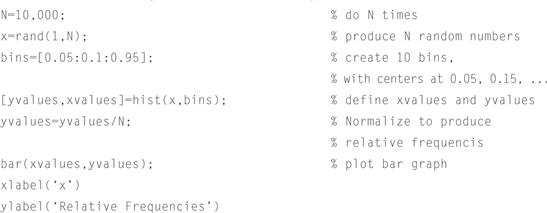
 The MATLAB function rand generates random numbers that are uniformly distributed in the interval (0, 1) using an algorithm which is discussed in Chapter 12. For the present, consider the algorithm to select a number from a table in a random like manner. To construct a histogram for the random numbers generated by rand we write a script that calls rand repeatedly. Since we can do this only a finite number of times, we quantize the range of the random numbers into increments of 0.1. We then calculate the number of times a random number falls in each quantized interval and divide by the total number of numbers generated for the example. If we plot this ratio of relative frequencies using a bar graph, the resulting plot is called a histogram. The MATLAB script for this example follows and the histogram is shown in Figure 3.4, where the total number of values generated is 10,000. Try changing the value of N or the number and width of the bins in this example to see how results vary.

Figure 3.4 Histogram of relative frequencies for a uniform random variable generated by MATLAB’s rand function using 10,000 trials.
3.3 The Gaussian Random Variable
In the study of random variables, the Gaussian random variable is the most commonly used and of most importance. As will be seen later in the text, many physical phenomenon can be modeled as Gaussian random variables, including the thermal noise encountered in electronic circuits. Although many students may not realize it, they are probably quite familiar with the Gaussian random variable, for it is this random variable which leads to the so-called curve on which many students are graded.
Definition 3.3: A Gaussian random variable is one whose PDF can be written in the general form
 (3.12)
The PDF of the Gaussian random variable has two parameters, m and σ, which have the interpretation of the mean and standard deviation, respectively.1 The parameter σ2 is referred to as the variance.
An example of a Guassian PDF is shown in Figure 3.5. In general, the Gaussian PDF is centered about the point x = m and has a width that is proportional to σ.

Figure 3.5 (a) PDF and (b) CDF of a Gaussian random variable with m = 3 and σ = 2.
It should be pointed out that in the mathematics and statistics literature, this random variable is referred to as a “normal” random variable. Furthermore, for the special case when m = 0 and σ = 1, it is called a “standard normal” random variable. However, in the engineering literature the term Gaussian is much more common, so this nomenclature will be used throughout this text.
Because Gaussian random variables are so commonly used in such a wide variety of applications, it is standard practice to introduce a shorthand notation to describe a Gaussian random variable, X ∼ N(m, σ2). This is read “X is distributed normally (or Gaussian) with mean, m, and variance, σ2.”
The first topic to be addressed in the study of Gaussian random variables is to find its CDF. The CDF is required whenever we want to find the probability that a Gaussian random variable lies above or below some threshold or in some interval. Using the relationship in Equation (3.11c), the CDF of a Gaussian random variable is written as
 (3.13)
It can be shown that it is impossible to express this integral in closed form. While this is unfortunate, it does not stop us from extensively using the Gaussian random variable. Two approaches can be taken to dealing with this problem. As with other important integrals that cannot be expressed in closed form (e.g., Bessel functions), the Gaussian CDF has been extensively tabulated and one can always look up values of the required CDF in a table, such as the one provided in Appendix E. However, it is often a better option to use one of several numerical routines which can approximate the desired integral to any desired accuracy.
The same sort of situation exists with many more commonly known mathematical functions. For example, what if a student was asked to find the tangent of 1.23 radians? While the student could look up the answer in a table of trig functions, that seems like a rather archaic approach. Any scientific calculator, high-level programming language, or math package will have internally generated functions to evaluate such standard mathematical functions. While not all scientific calculators and high-level programming languages have internally generated functions for evaluating Gaussian CDFs, most mathematical software packages do, and in any event, it is a fairly simple thing to write short program to evaluate the required function. Some numerical techniques for evaluating functions related to the Gaussian CDF are discussed specifically in Appendix F.
Whether the Gaussian CDF is to be evaluated by using a table or a program, the required CDF must be converted into one of a few commonly used standard forms. A few of these common forms are
The error function and its complement are most commonly used in the mathematics community; however, in this text, we will primarily use the Q-function. Nevertheless, students at least need to be familiar with the relationship between all of these functions because most math packages will have internally defined routines for the error function integral and perhaps its complement as well, but usually not the F-function or the Φ-function. So, why not just use error functions? The reason is that if one compares the integral expression for the Gaussian CDF in Equation (3.13) with the integral functions defined in our list, it is a more straightforward thing to express the Gaussian CDF in terms of a Φ-function or a Q-function. Also, the Q-function seems to be enjoying the most common usage in the engineering literature in recent years.
Perhaps the advantage of not working with error function integrals is clearer if we note that the Φ-function is simply the CDF of a standard normal random variable. For general Gaussian random variables which are not in the normalized form, the CDF can be expressed in terms of a Φ-function using a simple transformation. Starting with the Gaussian CDF in Equation (3.13), make the transformation t = (y-m)/σ, resulting in
 (3.14)
Hence, to evaluate the CDF of a Gaussian random variable, we just evaluate the Φ-function at the points (x – m)/σ.
The Q-function is more natural for evaluating probabilities of the form Pr(X > x). Following a line of reasoning identical to the previous paragraph, it is seen that if X ∼ N(m, σ2), then
 (3.15)
Furthermore, since we have shown that Pr(X > x) = Q((x – m)/σ) and Pr(X ≤ x) = Φ((x – m)/σ), it is apparent that the relationship between the Φ-function and the Q-function is
![]() (3.16)
(3.16)
This and other symmetry relationships can be visualized using the graphical definitions of the Φ-function (phi function) and the Q-function shown in Figure 3.6. Note that the CDF of a Gaussian random variable can be written in terms of a Q-function as
![]() (3.17)
(3.17)

Figure 3.6 Standardized integrals related to the Gaussian CDF: the Φ(.) and Q(.) functions.
Once the desired CDF has been expressed in terms of a Q-function, the numerical value can be looked up in a table or calculated with a numerical program. Other probabilities can be found in a similar manner as shown in the next example. It should be noted that some internally defined programs for Q and related functions may expect a positive argument. If it is required to evaluate the Q-function at a negative value, the relationship Q(x) = 1 – Q(–x) can be used. That is, to evaluate Q(−2), for example, Q(2) can be evaluated and then use Q(−2) = 1 – Q(2).
Example 3.7
A random variable has a PDF given by
![]()
Find each of the following probabilities and express the answers in terms of Q-functions.
For the given Gaussian PDF, m = −3 and σ = 2. For part (a),
![]()
This can be rewritten in terms of a Q-function as
![]()
The probability in part (b) is easier to express directly in terms of a Q-function.
![]()
In part (c), the probability of the random variable X falling in an interval is required. This event can be rewritten as
![]()
We can proceed in a similar manner for part (d).
![]()
Example 3.8
MATLAB has a built-in function, randn, which generates random variables according to a Gaussian or normal distribution. In particular, randn(k, n) creates an k × n matrix whose elements are randomly chosen according to a standard normal distribution. This example constructs a histogram of the numbers generated by the randn function similar to what was done in Example 3.6 using the rand function. Note that by multiplying the output of the randn function by σ and adding m, the Gaussian random variable produced by randn now has mean m and variance σ2. We will elaborate on such transformations and others in the next chapter. Note that the MATLAB code that follows is similar to that of Example 3.6 with the exception that we are now using randn instead of rand. Also the Gaussian PDF has a domain which is infinite and, thus, in principle we would need an infinite number of bins in our histogram. Since this is impractical, we chose a sufficiently large number of bins such that those not included would represent relatively insignificant values. Note also that in this histogram we are plotting probability densities rather than relative frequencies so that a direct comparison can be made between the histogram and the true PDF. The histogram obtained using the following code is shown in Figure 3.7.
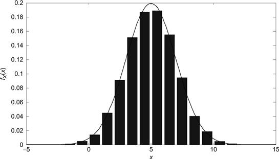
Figure 3.7 Histogram of random numbers produces by randn along with a Gaussian PDF; m = 5, σ = 2.


3.4 Other Important Random Variables
This section provides a summary of some other important random variables that find use in various engineering applications. For each random variable, an indication is given as to the sorts of applications that find use for these random variables.
3.4.1 Uniform Random Variable
The uniform PDF is constant over an interval [a, b). The PDF and its corresponding CDF are
 (3.18a)
 (3.18b)
Since this is a continuous random variable, the interval over which the PDF is nonzero can be open or closed on either end. A plot of the PDF and CDF of a uniform random variable is shown in Figure 3.8. Most computer random number generators will generate a random variable which closely approximates a uniform random variable over the interval (0, 1). We will see in the next chapter that by performing a transformation on this uniform random variable, we can create many other random variables of interest. An example of a uniform random variable would be the phase of a radio frequency sinusoid in a communication system. Although the transmitter knows the phase of the sinusoid, the receiver may have no information about the phase. In this case, the phase at the receiver could be modeled as a random variable uniformly distributed over the interval [0, 2π).

Figure 3.8 (a) Probability density function and (b) cumulative distribution function of a uniform random variable.
3.4.2 Exponential Random Variable
The exponential random variable has a PDF and CDF given by (for any b > 0)
![]() (3.19a)
(3.19a)
![]() (3.19b)
(3.19b)
A plot of the PDF and the CDF of an exponential random variable is shown in Figure 3.9. The parameter b is related to the width of the PDF and the PDF has a peak value of 1/b which occurs at x = 0. The PDF and CDF are nonzero over the semi-infinite interval (0,∞), which may be either open or closed on the left endpoint.

Figure 3.9 (a) Probability density function and (b) cumulative distribution function of an exponential random variable, b = 2.
Exponential random variables are commonly encountered in the study of queueing systems. The time between arrivals of customers at a bank, for example, is commonly modeled as an exponential random variable, as is the duration of voice conversations in a telephone network.
3.4.3 Laplace Random Variable
A Laplace random variable has a PDF which takes the form of a two-sided exponential. The functional forms of the PDF and CDF are given by (for any b > 0)
![]() (3.20a)
(3.20a)
 (3.20b)
A plot of these functions is shown in Figure 3.10. The width of the PDF is determined by the parameter b, while the peak value of the PDF is 1/2b. Note that this peak value is half of what it is in the case of the (one-sided) exponential shown in Figure 3.9. This makes sense since the Laplace random variable has two sides and the area under the curve must remain constant (and equal to unity). The Laplace random variable has been used to model the amplitude of a speech (voice) signal.

Figure 3.10 (a) Probability density function and (b) cumulative distribution function of a Laplace random variable, b = 2.
3.4.4 Gamma Random Variable
A random variable that follows a gamma distribution has a PDF and CDF given (for any b > 0 and any c > 0) by
![]() (3.21a)
(3.21a)
![]() (3.21b)
(3.21b)
In these two equations, the gamma function is a generalization of the factorial function defined by
![]() (3.22)
(3.22)
and the incomplete gamma function is given by
![]() (3.23)
(3.23)
The gamma random variable is used in queueing theory and has several other random variables as special cases. If the parameter c is an integer, the resulting random variable is also known as an Erlang random variable, whereas, if b = 2 and c is a half integer, a chi-squared (χ2) random variable results. Finally, if c = 1, the gamma random variable reduces to an exponential random variable.
3.4.5 Erlang Random Variable
As we have mentioned, the Erlang random variable is a special case of the gamma random variable. The PDF and CDF are given (for positive integer n and any b > 0) by
![]() (3.24)
(3.24)
 (3.25)
The Erlang distribution plays a fundamental role in the study of wireline telecommunication networks. In fact, this random variable plays such an important role in the analysis of trunked telephone systems that the amount of traffic on a telephone line is measured in Erlangs.
3.4.6 Chi-Squared Random Variable
Another special case of the gamma random variable, the chi-squared (χ2) random variable has a PDF and CDF given (for positive integer or half-integer values of c) by
![]() (3.26)
(3.26)
![]() (3.27)
(3.27)
Many engineering students are probably familiar with the χ2 random variable from previous studies of statistics. It also commonly appears in various detection problems.
3.4.7 Rayleigh Random Variable
A Rayleigh random variable, like the exponential random variable, has a one-sided PDF. The functional form of the PDF and CDF is given (for any σ > 0) by
![]() (3.28a)
(3.28a)
![]() (3.28b)
(3.28b)
Plots of these functions are shown in Figure 3.11. The Rayleigh distribution is described by a single parameter, σ2, which is related to the width of the Rayleigh PDF. In this case, the parameter σ2 is not to be interpreted as the variance of the Rayleigh random variable. It will be shown later that the Rayleigh distribution arises when studying the magnitude of a complex number whose real and imaginary parts both follow a zero-mean Gaussian distribution. The Rayleigh distribution arises often in the study of noncoherent communication systems and also in the study of wireless communication channels, where the phenomenon known as fading is often modeled using Rayleigh random variables.

Figure 3.11 (a) Probability density function and (b) cumulative distribution function of a Rayleigh random variable, σ2 = ½.
3.4.8 Rician Random Variable
A Rician random variable is closely related to the Rayleigh random variable (in fact the Rayleigh distribution is a special case of the Rician distribution). The functional form of the PDF for a Rician random variable is given (for any a > 0 and any σ > 0) by
![]() (3.29)
(3.29)
In this expression, the function Io(x) is the modified Bessel function of the first kind of order zero which is defined by
![]() (3.30)
(3.30)
Like the Gaussian random variable, the CDF of a Rician random variable cannot be written in closed form. Similar to the Q-function that is used to describe the Gaussian CDF, there is another function known as Marcum’s Q-function which describes the CDF of a Rician random variable. It is defined by
![]() (3.31)
(3.31)
The CDF of the Rician random variable is then given by:
![]() (3.32)
(3.32)
Tables of the Marcum Q-function can be found as well as efficient numerical routines for calculating it. A plot of the Rician PDF is shown in Figure 3.12. The Rician distribution is described by two parameters, a and σ2, which are related to the center and width, respectively, of the PDF. As with the Rayleigh random variable, the parameter σ2 is not to be interpreted as the variance of the Rician random variable. The Rician distribution arises in the study of noncoherent communication systems and also in the study of satellite communication channels, where fading is modeled using Rician random variables.

Figure 3.12 PDF of a Rician random variable, σ2 = 1/2, a = 1/2, 1, 2, 3.
3.4.9 Cauchy Random Variable
The Cauchy random variable has a PDF and CDF given (for any a and any b > 0) by
![]() (3.33)
(3.33)
![]() (3.34)
(3.34)
The Cauchy random variable occurs when observing the tangent of a random variable which is uniformly distributed over [0, 2π). The PDF is centered around x = a and its width is determined by the parameter b. Unlike most of the other random variables where the PDFs decrease exponentially in the tails, the Cauchy PDF decays quadratically as |x – a| increases. Hence, there is a greater amount of probability in the tails of the Cauchy PDF than in many of the other commonly used random variables. We say that this type of distribution is “heavy-tailed.”
Example 3.9
One can construct many new types of random variables by making functions of random variables. In this example, we construct a random variable which is the sine of a uniform random phase. That is, we construct a random variable which is uniformly distributed over [0, 2π) and then form a new random variable according to X = sin(Θ). In the next chapter, we will develop the tools to analytically figure out what the distribution of X should be, but for now we will simply observe its PDF by plotting a histogram. The MATLAB code below was used to accomplish this and the result is illustrated in Figure 3.13.

Figure 3.13 Histogram from Example 3.10, sine of a uniform phase.

3.5 Conditional Distribution and Density Functions
In Chapter 2, we defined the notion of conditional probability. In a similar manner, it is quite common to talk about the distribution or density of a random variable conditioned on some event, A. As with the initial study of random variables in the beginning of this chapter, it is convenient to start with the notion of a conditional CDF.
Definition 3.4: The conditional CDF of a random variable, X, conditioned on the event A having occurred is
![]() (3.35)
(3.35)
Naturally, this definition requires the caveat that the probability of the event A must not be zero.
The properties of CDFs listed in Equations (3.4a)–(3.4d) also apply to conditional CDFs, resulting in the following properties of conditional CDFs:
(1) ![]() (3.36a)
(3.36a)
(2) ![]() (3.36b)
(3.36b)
(3) ![]() (3.36c)
(3.36c)
(4) ![]() (3.36d)
(3.36d)
It is left as an exercise for the reader (see Exercise 3.13) to prove that these properties of CDFs do indeed apply to conditional CDFs as well.
Example 3.10
Suppose a random variable X is uniformly distributed over the interval [0,1) so that its CDF is given by
Suppose further that we want to find the conditional CDF of X given that X ≤ 1/2. Here, the event A = {X ≤ 1/2} is related to a numerical condition on the random variable itself. From the definition of a conditional CDF,
![]()
For x ≤ 0, the event X ≤ x has probability zero and hence FX|{X ≤ 1/2}(x) = 0 for x ≤ 0. When 0 ≤x≤ 1/2, the intersection of the events X ≤x and X ≤ 1/2 is simply the event X ≤x, so that
![]()
Finally, for x> 1/2, the intersection of the events X ≤ x and X ≤ 1/2 is simply the event X ≤ 1/2 and the conditional CDF reduces to one. Putting this all together, the desired conditional CDF is

In order to generalize the result of the previous example, suppose that for some arbitrary random variable X, the conditioning event is of the form A = a ≤ X ≤ b for some constants a ≤ b. Then
![]() (3.37)
(3.37)
If x ≤ a, then the events {X ≤ x} and a ≤ X ≤ b are mutually exclusive and the conditional CDF is zero. For x > b the event a ≤ X ≤ b is a subset of {X ≤ x} and hence Pr(X ≤ x, a ≤ X ≤ b) = Pr(a ≤ X ≤ b) so that the conditional CDF is 1. When a ≤ x ≤ b, then{X ≤ x} ∩ {a ≤ X ≤ b} = a ≤ X ≤ x and Pr(X ≤ x, a ≤ X ≤ b) = Pr(a ≤ X ≤ x). This can be written in terms of the CDF (unconditional) of X as Pr(a ≤ X ≤ x) = FX(x)−FX(a). Likewise, Pr(a ≤ X ≤ b) = FX(b)−FX(a). Putting these results together gives
 (3.38)
This result could also be extended to conditioning events where X is conditioned on being in more extravagant regions.
As with regular random variables, it is often more convenient to work with a conditional PDF rather than a conditional CDF. The definition of the conditional PDF is a straightforward extension of the previous definition given for a PDF.
Definition 3.5: The conditional PDF of a random variable X conditioned on some event A is
![]() (3.39)
(3.39)
As with the conditional CDF, it is not difficult to show that all of the properties of regular PDFs apply to conditional PDFs as well. In particular,
(1) ![]() (3.40a)
(3.40a)
(2)  (3.40b)
(3) ![]() (3.40c)
(3.40c)
(4) ![]() (3.40d)
(3.40d)
(5)  (3.40e)
Furthermore, the result in Equation (3.38) can be extended to the conditional PDF by applying Equation (3.40b). This results in the following general formula for the conditional PDF of a random variable, X, when the conditioning event is of the nature A = {a ≤ X ≤ b}:
 (3.41)
To summarize, the conditional PDF takes on the same functional form (but is scaled by the probability of the conditioning event) over the range of x where the condition is satisfied, and the conditional PDF is zero wherever the conditioning event is not true. This result is illustrated in Figure 3.14.

Figure 3.14 (a) A PDF and (b) the corresponding conditional PDF.
Example 3.11
Let X be a random variable representing the length of time we spend waiting in the grocery store checkout line. Suppose the random variable X has an exponential PDF given by fX(x) = (l/c)exp(–x/c)u(x), where c = 3 min. What is the PDF for the amount of time we spend waiting in line given that we have already been waiting for 2 min? Here the conditioning event is of the form X > 2. We can use the result in Equation (3.41) by taking a = 2 and b = ∞. The probability of the conditioning event is Pr(X > 2) = 1 –FX(2) = exp(−2/3). Therefore, the conditional PDF is
![]()
It is curious to note that for this example, fX|{x>2}(x) = fX(x−2). That is, given that we have been waiting in line for 2 min, the PDF of the total time we must wait in line is simply shifted by 2 min. This interesting behavior is unique to the exponential distribution and we might not have seen the same result if we had started with a different distribution. For example, try working the same problem starting with a Rayleigh distribution.
Up to this point, we have primarily looked at conditioning events that impose a numerical constraint. It is also common to consider conditioning events of a qualitative, or nonnumerical, nature. Consider, for example, a random variable X which represents a student’s score on a certain standardized test (e.g., the SAT or GRE test). We might be interested in determining if there is any gender bias in the test. To do so, we could compare the distribution of the variable X given that the student is female, FX|F(x), with the distribution of the same variable given that the student is male, FX|M(x). If these distributions are substantially different, then we might conclude a gender bias and work to fix the bias in the exam. Naturally, we could work with conditional PDFs fX|F(x) and fX|M(x) as well. Here, the conditioning event is a characteristic of the experiment that may affect the outcome rather than a restriction on the outcome itself.
In general, consider a set of mutually exclusive and exhaustive conditioning events, A1, A2, …, AN. Suppose we had access to the conditional CDFs, FX|A (x), n = 1, 2, …, N, and wanted to find the unconditional CDF, FX(x). According to the Theorem of Total Probability (Theorem 2.10),
 (3.42)
Hence, the CDF of X (unconditional) can be found by forming a weighted sum of the conditional CDFs with the weights determined by the probabilities that each of the conditioning events is true. By taking derivatives of both sides of the previous equation, a similar result is obtained for conditional PDFs, namely
 (3.43)
We might also be interested in looking at things in the reverse direction. That is, suppose we observe that the random variable has taken on a value of X = x. Does the probability of the event An change? To answer this we need to compute Pr(A|(X = x)). If X were a discrete random variable, we could do this by invoking the results of Theorem 2.5
![]() (3.44)
(3.44)
In the case of continuous random variables, greater care must be taken since both Pr(X = x|An) and Pr(X = x) will be zero, resulting in an indeterminate expression. To avoid that problem, rewrite the event {X = x} as{x ≤ X ≤ x + ε} and consider the result in the limit as ε → 0:
![]() (3.45)
(3.45)
Note that for infinitesimal ε, Pr(x ≤ X ≤ x + ε) = fx(x)ε and similarly ![]() . Hence,
. Hence,
 (3.46)
Finally, passing to the limit as ε → 0 gives the desired result:
 (3.47)
We could also combine this result with Equation (3.43) to produce an extension to Bayes’s theorem:
 (3.48)
Example 3.12
In a certain junior swimming competition, swimmers are placed into one of two categories based on their previous times so that all children can compete against others of their own abilities. The fastest swimmers are placed in the A category, while the slower swimmers are put in the B group. Let X be a random variable representing a child’s time (in seconds) in the 50-m freestyle race. Suppose that it is determined that for those swimmers in group A, the PDF of a child’s time is given by fx|A(x) = (4π)−1/2exp(–(x−40)2/4) while for those in the B group the PDF is given by fx|B(x) = (4π)−1/2exp(–(x−45)2/4). Furthermore, assume that 30% of the swimmers are in the A group and 70% are in the B group. If a child swims the race with a time of 42 s, what is the probability that the child was in the B group? Applying Equation (3.48) we get
![]()
Naturally, the probability of the child being from group A must then be
![]()
3.6 Engineering Application: Reliability and Failure Rates
The concepts of random variables presented in this chapter are used extensively in the study of system reliability. Consider an electronic component that is to be assembled with other components as part of a larger system. Given a probabilistic description of the lifetime of such a component, what can we say about the lifetime of the system itself. The concepts of reliability and failure rates are introduced in this section to provide tools to answer such questions.
Definition 3.6: Let X be a random variable which represents the lifetime of a device. That is, if the device is turned on at time zero, X would represent the time at which the device fails. The reliability function of the device, RX (t), is simply the probability that the device is still functioning at time t:
![]() (3.49)
(3.49)
Note that the reliability function is just the complement of the CDF of the random variable. That is, RX (t) = 1 – FX (t). As it is often more convenient to work with PDFs rather than CDFs, we note that the derivative of the reliability function can be related to the PDF of the random variable X by RX‘(t) = – f X (t).
With many devices, the reliability changes as a function of how long the device has been functioning. Suppose we observe that a particular device is still functioning at some point in time t. The remaining lifetime of the device may behave (in a probabilistic sense) very differently from when it was first turned on. The concept of failure rate is used to quantify this effect.
Definition 3.7: Let X be a random variable which represents the lifetime of a device. The failure rate function is
![]() (3.50)
(3.50)
To give this quantity some physical meaning, we note that Pr(t ≤ X ≤ t + dt X > t) = r(t)dt. Thus, r(t)dt is the probability that the device will fail in the next time instant of length dt, given the device has survived up to now (time t). Different types of “devices” have failure rates that behave in different manners. Our pet goldfish, Elvis, might have an increasing failure rate function (as do most biological creatures). That is, the chances of Elvis “going belly up” in the next week is greater when Elvis is 6 months old than when he is just 1 month old. We could also imagine devices that have a decreasing failure rate function (at least for part of their lifetime). For example, an integrated circuit might be classified into one of two types, those which are fabricated correctly and hence are expected to have a quite long lifetime and those with defects which will generally fail fairly quickly. When we select an IC, we may not know which type it is. Once the device lives beyond that initial period when the defective ICs tend to fail, the failure rate may go down (at least for awhile). Finally, there may be some devices whose failure rates remain constant with time.
The failure rate of a device can be related to its reliability function. From Equation (3.41) it is noted that
 (3.51)
The denominator in the above expression is the reliability function, RX (t), while the PDF in the numerator is simply –RX‘(x). Evaluating at x = t produces the failure rate function
 (3.52)
Conversely, given a failure rate function, r(t), one can solve for the reliability function by solving the first-order differential equation:
![]() (3.53)
(3.53)
The general solution to this differential equation (subject to the initial condition Rx (0) = 1) is
![]() (3.54)
(3.54)
It is interesting to note that a failure rate function completely specifies the PDF of a device’s lifetime:
![]() (3.55)
(3.55)
For example, suppose a device had a constant failure rate function, r(t) = λ. The PDF of the device’s lifetime would then follow an exponential distribution, fx(t) = λ exp(–λ t)u(t). The corresponding reliability function would also be exponential, RX(t) = exp(–λ t)u(t). We say that the exponential random variable has the memoryless property. That is, it does not matter how long the device has been functioning, the failure rate remains the same.
Example 3.13
Suppose the lifetime of a certain device follows a Rayleigh distribution given by fx(t) = 2bt exp(–bt2)u(t). What are the reliability function and the failure rate function? The reliability function is given by
![]()
A straightforward application of Equation (3.52) produces the failure rate function, r(t) = 2btu(t). In this case, the failure rate is linearly increasing in time.
Next, suppose we have a system which consists of N components, each of which has a lifetime described by the random variable Xn, n = 1, 2, …, N. Furthermore, assume that for the system to function, all N components must each be functioning. In other words, if any of the individual components fail, the whole system fails. This is usually referred to as a series connection of components. If we can characterize the reliability and failure rate functions of each individual component, can we calculate the same functions for the entire system? The answer is yes, under some mild assumptions. Define X to be the random variable representing the lifetime of the system. Then
![]() (3.56)
(3.56)
Furthermore,

We assume that all of the components fail independently. That is, the event {Xi > t} is taken to be independent of {X j > t} for all i ≠ j. Under this assumption,
 (3.58)
Furthermore, application of Equation (3.52) provides an expression for the failure rate function:
 (3.59)
 (3.60)
where rn (t) is the failure rate function of the nth component. We have shown that for a series connection of components, the reliability function of the system is the product of the reliability functions of each component and the failure rate function of the system is the sum of the failure rate functions of the individual components.
We may also consider a system which consists of a parallel interconnection of components. That is, the system will be functional as long as any of the components are functional. We can follow a similar derivation to compute the reliability and failure rate functions for the parallel interconnection system. First, the reliability function is written as
![]() (3.61)
(3.61)
In this case, it is easier to work with the complement of the reliability function (the CDF of the lifetime). Since the reliability function represents the probability that the system is still functioning at time t, the complement of the reliability function represents the probability that the system is not working at time t. With the parallel interconnections, the system will fail only if all the individual components fail. Hence,
 (3.62)
As a result, the reliability function of the parallel interconnection system is given by
 (3.63)
Unfortunately, the general formula for the failure rate function is not as simple as in the serial interconnection case. Application of Equation (3.52) to our preceding equation gives (after some straightforward manipulations)
 (3.64)
or, equivalently,
 (3.65)
Example 3.14
Suppose a system consists of N components each with a constant failure rate, rn(t) = λn, n = 1, 2, …, N. Find the reliability and failure rate functions for a series interconnection.
Then find the same functions for a parallel interconnection. It was shown previously that a constant failure rate function corresponds to an exponential reliability function.
That is, ![]() For the serial interconnection we then have
For the serial interconnection we then have

For the parallel interconnection,

Exercises
Section 3.1: The Cumulative Distribution Function
3.1 Which of the following mathematical functions could be the CDF of some random variable?

3.2 Suppose a random variable has a CDF given by
![]()
Find the following quantities:
3.3 Repeat Exercise 3.2 for the case where the random variable has the CDF
![]()
3.4 Suppose we flip a balanced coin five times and let the random variable X represent the number of times heads occurs.
3.5 A random variable is equally likely to take on any integer value in the set { 0, 1, 2, 3 }.
3.6 A certain discrete random variable has a CDF given by

(a) Find the probability mass function, PX(k), of this random variable.
(b) For a positive integer n, find Pr(X ⊂ n).
(c) For two positive integers, n1and n2, such that nl≤n2, find Pr(n1 ≤ X ≤ n2).
3.7 In this problem, we generalize the results of Exercise 3.6. Suppose a discrete random variable takes on nonnegative integer values and has a CDF of the general form
(a) What conditions must the sequence ak satisfy for this to be a valid CDF.
(b) For a positive integer n, find Pr(X ≤ n) in terms of the ak.
3.8 A random variable has a CDF given by FX(x) = (l–e−x)u(x).
3.9 A random variable has a CDF given by

Section 3.2: The Probability Density Function
3.10 Suppose a random variable is equally likely to fall anywhere in the interval [a, b]. Then the PDF is of the form
Find and sketch the corresponding CDF.
3.11 Find and plot the CDFs corresponding to each of the following PDFs:


3.12 A random variable has the following exponential PDF:

where a and b are constants.
3.13 A certain random variable has a probability density function of the form f X (x) = ce−2xu(x). Find the following:
3.14 Repeat Exercise 3.13 using the PDF ![]()
3.15 Repeat Exercise 3.13 using the PDF ![]()
3.16 The voltage of communication signal S is measured. However, the measurement procedure is corrupted by noise resulting in a random measurement with the PDF shown in the accompanying diagram. Find the probability that for any particular measurement, the error will exceed ±0.75 % of the correct value if this correct value is 10 V.

3.17 Which of the following mathematical functions could be the PDF of some random variable?


3.18 Find the value of the constant c that makes each of the following functions a properly normalized PDF.

Section 3.3: The Gaussian Random Variable
3.19 Prove the integral identity, ![]() Hint: It may be easier to show that I2 = 2π.
Hint: It may be easier to show that I2 = 2π.
3.20 Using the normalization integral for a Gaussian random variable, find an analytical expression for the following integral:
![]()
where a> 0, b, and c are constants.
3.21 A Gaussian random variable has a probability density function of the form
![]()
(a) Find the value of the constant c.
(b) Find the values of the parameters m and σ for this Gaussian random variable.
3.22 A Gaussian random variable has a PDF of the form
![]()
Write each of the following probabilities in terms of Q-functions (with positive arguments) and also give numerical evaluations:
3.23 A Gaussian random variable has a PDF of the form
![]()
Write each of the following probabilities in terms of Q-functions (with positive arguments) and also give numerical evaluations:
3.24 Suppose we measure the noise in a resistor (with no applied voltage) and find that the noise voltage exceeds 10 μV 5% of the time. We have reason to believe the noise is well modeled as a Gaussian random variable, and furthermore, we expect the noise to be positive and negative equally often so we take the parameter, m, in the Gaussian PDF to be m = 0. Find the value of the parameter, σ2. What units should be associated with σ2 in this case.
3.25 Now suppose we modify Exercise 3.24 so that in addition to noise in the resistor there is also a weak (constant) signal present. Thus, when we measure the voltage across the resistor, we do not necessarily expect positive and negative measurements equally often, and therefore, we now allow the parameter m to be something other than zero. Suppose now we observe that the measure voltage exceeds 10 μV 40% of the time and is below−10 μV only 2% of the time. If we continue to model the voltage across the resistor as a Gaussian random variable, what are the appropriate values of the parameters m and σ2. Give proper units for each.
3.26 The IQ of a randomly chosen individual is modeled using a Gaussian random variable. Given that 50% of the population have an IQ above 100 (and 50% have an IQ below 100) and that 50% of the population have an IQ in the range 90-100, what percentage of the population have an IQ of at least 140 and thereby are considered “genius?”
Section 3.4: Other Important Random Variables
3.27 The phase of a sinusoid, Θ, is uniformly distributed over [0, 2π) so that its PDF is of the form

3.28 Let X be an exponential random variable with PDF, f X (x) = e−x u(x).
(b) Generalize your answer to part (a) to find Pr(3 X ≤ y) for some arbitrary constant y.
(c) Note that if we define a new random variable according to Y = 3X, then your answer to part (b) is the CDF of Y, FY(y). Given your answer to part (b), find f Y(y).
3.29 Let W be a Laplace random variable with a PDF given by fw(w) = ce−2|w|.
3.30 Let Z be a random variable whose PDF is given by fz(z) = cz2 e−zu(z).
3.31 Let R be a Rayleigh random variable whose PDF is fR(r) = crexp(− r2)u(r).
3.32 A random variable, Y, has a PDF given by
![]()
Section 3.5: Conditional Distribution and Density Functions
3.34 Prove the following properties of conditional CDFs.
3.35 Let X be a Gaussian random variable such that X ∼ N(0, σ2). Find and plot the following conditional PDFs.
3.36 A digital communication system sends two messages, M = 0 or M = 1, with equal probability. A receiver observes a voltage which can be modeled as a Gaussian random variable, X, whose PDFs conditioned on the transmitted message are given by
![]()
(a) Find and plot Pr(M = 0|X = x) as a function of x for σ2 = 1. Repeat for σ2 = 5.
(b) Repeat part (a) assuming that the a priori probabilities are Pr(M = 0) = 1/4 and Pr(M = l) = 3/4.
3.37 In Exercise 3.36, suppose our receiver must observe the random variable X and then make a decision as to what message was sent. Furthermore, suppose the receiver makes a three-level decision as follows:
Decide 0 was sent if Pr(M= 0|X=x) ≥ 0.9,
Decide 1 was sent if Pr(M= l|X=x) ≥ 0.9,
Erase the symbol (decide not to decide) if both Pr(M = 0|X=x) ≤ 0.9 and Pr(M = l|X = x)≤0.9.
Assuming the two messages are equally probable, Pr(M = 0) = Pr(M = 1) = 1/2, and that σ2 = 1, find
(a) the range of x over which each of the three decisions should be made,
(b) the probability that the receiver erases a symbol,
(c) the probability that the receiver makes an error (i.e., decides a “0” was sent when a “1” was actually sent, or vice versa).
3.38 In this problem, we extend the results of Exercise 3.36 to the case when there are more than two possible messages sent. Suppose now that the communication system sends one of four possible messages M = 0, M = 1, M = 2, and M = 3, each with equal probability. The corresponding conditional PDFs of the voltage measured at the receiver are of the form
![]()
(a) Find and plot Pr(M = m | X = x) as a function of x for σ2 = 1.
(b) Determine the range of x for which Pr(M =0|X = x) > Pr(M =m|X= x) for all m ≠ 0. This will be the range of x for which the receiver will decide in favor of the message M = 0.
(c) Determine the range of x for which Pr(M = 1|X = x) > Pr(M = m|X = x) for all m ≠ 1. This will be the range of x for which the receiver will decide in favor of the message M = 1.
(d) Based on your results of parts (b) and (c) and the symmetry of the problem, can you infer the ranges of x for which the receiver will decide in favor of the other two messages, M = 2 and M = 3?
3.39 Suppose V is a uniform random variable,

3.40 Repeat Exercise 3.39 if V is a Rayleigh random variable with PDF,
![]()
Section 3.6: Reliability and Failure Rates
3.41 Recalling Example 3.14, suppose that a serial connection system has 10 components and the failure rate function is the same constant for all components and is 1 per 100 days.
Miscellaneous Exercises
3.42 Mr. Hood is a good archer. He can regularly hit a target having a 3-ft. diameter and often hits the bull’s-eye, which is 0.5 ft. in diameter, from 50 ft. away. Suppose the miss is measured as the radial distance from the center of the target and, furthermore, that the radial miss distance is a Rayleigh random variable with the constant in the Rayleigh PDF being σ2 = 4 (sq-ft).
(a) Determine the probability of Mr. Hood’s hitting the target.
(b) Determine the probability of Mr. Hood’s hitting the bull’s-eye.
(c) Determine the probability of Mr. Hood’s hitting the bull’s-eye given that he hits the target.
3.43 In this problem, we revisit the light bulb problem of Exercise 2.74. Recall that there were two types of light bulbs, long-life (L) and short-life (S) and we were given an unmarked bulb and needed to identify which type of bulb it was by observing how long it functioned before it burned out. Suppose we modify the problem so that the lifetime of the bulbs are modeled with a continuous random variable. In particular, suppose the two conditional PDFs are now given by
![]()
where X is the random variable that measures the lifetime of the bulb in hours. The a priori probabilities of the bulb type were Pr(S) = 0.75 and Pr(L) = 0.25.
(a) If a bulb is tested and it is observed that the bulb burns out after 200 h, which type of bulb was most likely tested?
(b) What is the probability that your decision in part (a) was incorrect?
3.44 Consider the light bulb problem in Exercise 3.43. Suppose we do not necessarily want to wait for the light bulb to burn out before we make a decision as to which type of bulb is being tested. Therefore, a modified experiment is proposed. The light bulb to be tested will be turned on at 5 pm on Friday and will be allowed to burn all weekend. We will come back and check on it Monday morning at 8 am and at that point it will either still be lit or it will have burned out. Note that since there are a total of 63 h between the time we start and end the experiment and we will not be watching the bulb at any point in time in between, there are only two possible observations in this experiment, (the bulb burnt out ⇔ {X ≤ 63 }) or (the bulb is still lit ⇔ {X > 63 }).
(a) Given it is observed that the bulb burnt out over the weekend, what is the probability that the bulb was an S-type bulb?
(b) Given it is observed that the bulb is still lit at the end of the weekend, what is the probability that the bulb was an S type bulb?
3.45 Suppose we are given samples of the CDF of a random variable. That is, we are given Fn = Fx(xn) at several points, xn ∈ {x1, x2, x3, …, xk}. After examining a plot of the samples of the CDF, we determine that it appears to follow the functional form of a Rayleigh CDF,
The object of this problem is to determine what value of the parameter, σ2, in the Rayleigh CDF best fits the given data.
(a) Define the error between the n th sample point and the model to be
![]()
Find an equation that the parameter σ2 must satisfy if it is to minimize the sum of the squared errors,

Note, you probably will not be able to solve this equation, you just need to set up the equation.
(b) Next, we will show that the optimization works out to be analytically simpler if we do it in the log domain and if we work with the complement of the CDF. That is, suppose we redefine the error between the nth sample point and the model to be
![]()
Find an equation that the parameter σ2 must satisfy if it is to minimize the sum of the squared errors. In this case, you should be able to solve the equation and find an expression for the optimum value of σ2.
MATLAB Exercises
3.46 Write a MATLAB program to calculate the probability Pr(x1 ≤ X ≤ x2) if X is a Gaussian random variable for an arbitrary x1 and x2. Note you will have to specify the mean and variance of the Gaussian random variable.
3.47 Write a MATLAB program to calculate the probability Pr(|X – a|≤ b) if X is a Gaussian random variable for an arbitrary a and b > 0. Note you will have to specify the mean and variance of the Gaussian random variable.
3.48 Use the MATLAB rand function to create a random variable X uniformly distributed over (0, 1). Then create a new random variable according to Y = –ln(X). Repeat this procedure many times to create a large number of realizations of Y. Using these samples, estimate and plot the probability density function of Y. Find an analytical model that seems to fit your estimated PDF.
3.49 Use the MATLAB randn function to create a Gaussian distributed random variable X. Repeat this procedure and form a new random variable Y. Finally, form a random variable Z according to ![]() . Repeat this procedure many times to create a large number of realizations of Z. Using these samples, estimate and plot the probability density function of Z. Find an analytical model that seems to fit your estimated PDF.
. Repeat this procedure many times to create a large number of realizations of Z. Using these samples, estimate and plot the probability density function of Z. Find an analytical model that seems to fit your estimated PDF.
3.50 Use the MATLAB randn function to generate a large number of samples generated according to a Gaussian distribution. Let A be the event A = {the sample is greater than 1.5}. Of those samples that are members of the event A, what proportion (relative frequency) is greater than 2. By computing this proportion you will have estimated the conditional probability Pr(X > 2|X > 1.5). Calculate the exact conditional probability analytically and compare it with the numerical results obtained through your MATLAB program.
3.51 Write a MATLAB program to evaluate the inverse of a Q-function. That is, if the program is input a number, x, subject to 0 ≤ x ≤ 1, it will produce an output y = Q−1(x) which is the solution to Q(y) = x.
3.52 Use the MATLAB function marcumq to write a program to plot the CDF of a Rician random variable. Your program should take as inputs the two parameters a and σ of the Rician random variable and output a plot of the CDF. Be sure to correctly label the axes on your plot.
1 The terms mean, standard deviation, and variance will be defined and explained carefully in the next chapter.