
CHAPTER 11
Random Processes in Linear Systems
In this chapter, we consider the response of both continuous time and discrete-time linear systems to random processes, such as a signal plus noise. We develop statistical descriptions of the output of linear systems with random inputs by viewing the systems in both the time domain and the frequency domain. An engineering application section at the end of this chapter demonstrates how filters can be optimized for the purpose of enhancing signal-to-noise ratios. It is assumed that the reader is familiar with the study of linear time-invariant (LTI) systems. A brief overview is provided in Appendix C for those needing a refresher.
11.1 Continuous Time Linear Systems
Consider a linear time-invariant (LTI) system described by an impulse response h (t) or a transfer function H(f). If a random process, X(t), is the input to this system, the output will also be random and is given by the convolution integral
![]() (11.1)
(11.1)
We would like to statistically describe the output of the system. Ultimately, the joint PDF of any number of samples of the output would be nice. In general, this is a very difficult problem and hence we have to be satisfied with a simpler description. However, if the input process is Gaussian, then the output process will also be Gaussian, since any linear processing of Gaussian random variables (processes) produces new Gaussian random variables (processes). In that case, to completely describe the output of the system, we need merely to compute the mean and the autocovariance (or autocorrelation) function of the output. Even if the processes involved are not Gaussian, the mean and autocorrelation functions will serve as a good start toward describing the process. Therefore, our first goal will be to specify the mean and autocorrelation functions of the output of an LTI system with a random input.
To start with, consider the mean function of the output:
 (11.2)
Therefore, the output mean is the convolution of the input mean process with the impulse response of the system. For the special case when the input is wide sense stationary (WSS) and the input mean function is thereby constant, the output mean function becomes
![]() (11.3)
(11.3)
Note that the mean function of the output is also constant provided the input mean is constant. The autocorrelation function of the output is calculated in a similar manner.
 (11.4)
For WSS inputs, this expression can be simplified a little by using the fact that Rxx (u, v) = Rxx (v − u). The output autocorrelation function is then
![]() (11.5)
(11.5)
Although it may not appear like it from this expression, here, the output autocorrelation function is also a function of time difference only. To see this, perform the change of variables s = t1 − u and w = t2−v. Then Equation (11.5) becomes
![]() (11.6)
(11.6)
Now it is clear that RYY (t1,t2) = RYY (t2 − t1). To write this result in a more compact form, note that the inner integral in Equation (11.6) can be expressed as
![]() (11.7)
(11.7)
where * denotes convolution. Let g(t) =RXX (t) * h (t), then the output autocorrelation can be expressed as
![]() (11.8)
(11.8)
Putting all these results together, we get
![]() (11.9)
(11.9)
Thus, the output autocorrelation function is found by a double convolution. The presence of the double convolution in the previous equation begs for an equivalent frequency domain representation. Taking Fourier transforms of both sides gives an expression for the power spectral density (PSD) of the output of the filter in terms of the input PSD:
![]() (11.10)
(11.10)
The term |H(f)|2 is sometimes referred to as the power transfer function because it describes how the power is transferred from the input to the output of the system. In summary, we have shown the following results.
Theorem 11.1: Given an LTI system with impulse response h (t) or transfer function H(f) and a random input process X(t), the mean and autocorrelation functions of the output process, Y(t), can be described by
![]() (11.11a)
(11.11a)
![]() (11.11b)
(11.11b)
Furthermore, if X(t) is WSS, then Y(t) is also WSS with
![]() (11.12a)
(11.12a)
![]() (11.12b)
(11.12b)
![]() (11.12c)
(11.12c)
At times, it is desirable to specify the relationship between the input and output of a filter. Toward that end, we can calculate the cross-correlation function between the input and output.
 (11.13)
If X(t) is WSS, then this simplifies to
![]() (11.14)
(11.14)
In a similar manner, it can be shown that
![]() (11.15)
(11.15)
In terms of cross-spectral densities, these equations can be written as
![]() (11.16)
(11.16)
Example 11.1
White Gaussian noise, N(t), with a PSD of SNN (f) = No/2 is input to an RC lowpass filter (LPF). Such a filter will have a transfer function and impulse response given by
![]()
respectively. If the input noise is zero-mean, μN = 0, then the output process will also be zero-mean, μY = 0. Also
![]()
Using inverse Fourier transforms, the output autocorrelation is found to be
![]()
Example 11.2
Suppose we wish to convert a white noise process from continuous time to discrete time using a sampler. Since white noise has infinite power, it cannot be sampled directly and must be filtered first. Suppose for simplicity we use an ideal LPF of bandwidth B to perform the sampling so that the system is as illustrated in Figure 11.1. Let Nf (t) be the random process at the output of the LPF. This process has a PSD of
![]()

Figure 11.1 Block diagram of a sampling system to convert white noise from continuous time to discrete time.
The corresponding autocorrelation function is
![]()
If the output of the filter is sampled every to seconds, the discrete-time noise process will have an autocorrelation of RNN [k] = NoBsinc(2kBto ). If the discrete-time output process N[n] is to be white, then we want all samples to be uncorrelated. That is, we want RNN [k] = 0 for all k# 0. Recall that the sinc function has nulls whenever its argument is an integer. Thus, the discrete-time process will be white if (and only if) 2Bto is an integer. In terms of the sampling rate, fo = 1 /to , for the discrete-time process to be white, the sampling rate must be fo = 2B/m for some integer m.
11.2 Discrete-Time Linear Systems
The response of a discrete-time linear system to a (discrete-time) random process is found using virtually identical techniques to those used with continuous time systems. As such, we do not repeat the derivations here, but rather summarize the relevant results. We start with a linear system described by the difference equation
 (11.17)
where X[n] is the input to the system and Y[n] is the output. The reader might recognize this system as producing an autoregressive moving average process as described in Section 10.4. This system can be described by a transfer function expressed using either z-transforms or discrete-time Fourier transforms (DTFT) as
 (11.18)
If the DTFT is used, it is understood that the frequency variable f is actually a normalized frequency (normalized by the sampling rate). The system can also be described in terms of a discrete-time impulse response, h [n], which can be found through either an inverse z-transform or an inverse DTFT. The following results apply to any discrete-time system described by an impulse response, h[n], and transfer function, H(f).
Theorem 11.2: Given a discrete-time LTI system with impulse response h[n] and transfer function H(f), and a random input process X[n], the mean and autocorrelation functions of the output process, Y[n], can be described by
![]() (11.19a)
(11.19a)
 (11.19b)
Furthermore, if X[n] is WSS, then Y[n] is also WSS with
![]() (11.20a)
(11.20a)
![]() (11.20b)
(11.20b)
![]() (11.20c)
(11.20c)
Again, it is emphasized that the frequency variable in the PSD of a discrete-time process is to be interpreted as frequency normalized by the sampling rate.
Example 11.3
A discrete-time Gaussian white noise process has zero-mean and an autocorrelation function of RXX [n] = a2 δ[n]. This process is input to a system described by the difference equation
![]()
Note that this produces an AR(1) process at the output. The transfer function and impulse response of this system are
![]()
respectively, assuming that |a| ≤ 1. The autocorrelation and PSD functions of the output process are
![]()
respectively.
11.3 Noise Equivalent Bandwidth
Consider an ideal LPF with a bandwidth B whose transfer function is shown in Figure 11.2. Suppose white Gaussian noise with PSD No/ 2 is passed through this filter. The total output power would be Po = No B. For an arbitrary LPF, the output noise power would be
 (11.21)

Figure 11.2 Power transfer function of an arbitrary and ideal LPF. B = Bne if areas under the two curves are equal.
One way to define the bandwidth of an arbitrary filter is to construct an ideal LPF that produces the same output power as the actual filter. This results in the following definition of bandwidth known as noise equivalent bandwidth.
Definition 11.1: The noise equivalent bandwidth of a LPF with transfer function H(f) is
![]() (11.22)
(11.22)
This definition needs to be slightly adjusted for bandpass filters (BPFs). If the center of the passband is taken to be at some frequency, fo , then the noise equivalent bandwidth is
 (11.23)
Example 11.4
Consider the RC LPF whose transfer function is
![]()
The noise equivalent bandwidth of this filter is
![]()
In addition to using the noise equivalent bandwidth, the definitions in Section 10.3 presented for calculating the bandwidth of a random process can also be applied to find the bandwidth of a filter. For example, the absolute bandwidth and the RMS bandwidth of this filter are both infinite while the 3 dB (half power) bandwidth of this filter is
![]()
which for this example is slightly smaller than the noise equivalent bandwidth.
11.4 Signal-to-Noise Ratios
Often the input to a linear system will consist of signal plus noise, namely,
![]() (11.24)
(11.24)
where the signal part can be deterministic or a random process. We can invoke linearity to show that the mean process of the output can be viewed as a sum of the mean due to the signal input alone plus the mean due to the noise input alone. That is,
![]() (11.25)
(11.25)
In most cases, the noise is taken to be zero-mean, in which case the mean at the output is due to the signal part alone.
When calculating the autocorrelation function of the output, we cannot invoke superposition since autocorrelation is not a linear operation. First, we calculate the autocorrelation function of the signal plus noise input.
![]() (11.26)
(11.26)
If the signal and noise part are independent, which is generally a reasonable assumption, and the noise is zero-mean, then this autocorrelation becomes
![]() (11.27)
(11.27)
or, assuming all processes involved are WSS,
![]() (11.28)
(11.28)
As a result, the PSD of the output can be written as
![]() (11.29)
(11.29)
which is composed of two terms, namely that due to the signal and that due to the noise. We can then calculate the output power due to the signal part and the output power due to the noise part.
Definition 11.2: The signal-to-noise ratio (SNR) for a signal comprises the sum of a desired (signal) part and a noise part is defined as the ratio of the power of the signal part to the power (variance) of the noise part. That is, for X(t) = S(t) + N(t),
 (11.30)
Example 11.5
Suppose the input to the RC LPF of the previous example consists of a sinusoidal signal plus white noise. That is, let the input be X(t) = S(t) + N(t), where N(t) is white Gaussian noise as in the previous example and S(t) = acos (ωot + Θ), where Θ is a uniform random variable over [0, 2π) that is independent of the noise. The output can be written as Y(t)= So (t)+ No (t), where So (t) is the output due to the sinusoidal signal input and No (t) is the output due to the noise. The signal output can be expressed as
![]()
and the power in this sinusoidal signal is
![]()
From the results of Example 11.1, the noise power at the output is
![]()
Therefore, the SNR of the output of the RC LPF is
![]()
Suppose we desire to adjust the RC time constant (or, equivalently, adjust the bandwidth) of the filter so that the output SNR is optimized. Differentiating with respect to the quantity RC, setting equal to zero and solving the resulting equation produces the optimum time constant
![]()
Stated another way, the 3 dB frequency of the RC filter is set equal to the frequency of the input sinusoid in order to optimize output SNR. The resulting optimum SNR is
![]()
11.5 The Matched Filter
Suppose we are given an input process consisting of a (known, deterministic) signal plus an independent white noise process (with a PSD of No /2). It is desired to filter out as much of the noise as possible while retaining the desired signal. The general system is shown in Figure 11.3. The input process X(t) = s(t) + N(t) is to be passed through a filter with impulse response h (t) that produces an output process Y(t). The goal here is to design the filter to maximize the SNR at the filter output. Due to the fact that the input process is not necessarily stationary, the output process may not be stationary and therefore the output SNR may be time varying. Hence, we must specify at what point in time we want the SNR to be maximized. Picking an arbitrary sampling time, to , for the output process, we desire to design the filter such that the SNR is maximized at time t=to .
![]()
Figure 11.3 Linear system for filtering noise from a desired signal.
Let Yo be the value of the output of the filter at time to . This random variable can be expressed as
![]() (11.31)
(11.31)
where NY (t) is the noise process out of the filter. The powers in the signal and noise parts, respectively, are given by
 (11.32)
 (11.33)
The SNR is then expressed as the ratio of these two quantities,
 (11.34)
We seek the impulse response (or equivalently the transfer function) of the filter that maximizes the SNR as given in Equation (11.34). To simplify this optimization problem, we use Schwarz’s inequality, which states that
 (11.35)
where equality holds if and only if x(t) ∞ y (t)1. Applying this result to the expression for SNR produces an upper bound on the SNR:
 (11.36)
where Es is the energy in the signal s (t). Furthermore, this maximum SNR is achieved when h (t) ∞ s (to − t). In terms of the transfer function, this relationship is expressed as H(f) ∞ S*(f)e−J2πfto. The filter that maximizes the SNR is referred to as a matched filtersince the impulse response is matched to that of the desired signal. These results are summarized in the following theorem.
Theorem 11.3: If an input to an LTI system characterized by an impulse response, h(t), is given by X(t) = s(t) + N(t) where N(t) is a white noise process, then a matched filter will maximize the output SNR at time to . The impulse response and transfer function of the matched filter are given by
![]() (11.37)
(11.37)
Furthermore, if the white noise at the input has a PSD of SNN (f) = No/ 2, then the optimum SNR produced by the matched filter is
 (11.38)
where Es is the energy in the signal s (t).
Example 11.6
A certain communication system transmits a square pulse given by
![]()
This signal is received in the presence of white noise at a receiver producing the received process R(t) = s(t) + N(t). The matched filter that produces the optimum SNR at time to for this signal has an impulse response of the form
![]()
The output of the matched filter is then given by
![]()
Therefore, the matched filter for a square pulse is just a finite time integrator. The matched filter simply integrates the received signal for a period of time equal to the width of the pulse. When sampled at the correct point in time, the output of this integrator will produce the maximum SNR. The operation of this filter is illustrated in Figure 11.4.

Figure 11.4 (a) A square pulse, (b) the corresponding matched filter, and (c) the response of the matched filter to the square pulse.
Example 11.7
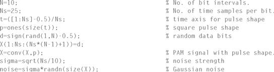
 In this example, we expand on the results of the previous example and consider a sequence of square pulses with random (binary) amplitudes as might be transmitted in a typical communication system. Suppose this signal is corrupted by white Gaussian noise and we must detect the transmitted bits. That is, we must determine whether each pulse sent has a positive or negative amplitude. Figure 11.5a shows both the square pulse train and the same signal corrupted by noise. Note that by visually observing the signals, it is very difficult to make out the original signal from the noisy version. We attempt to clean up this signal by passing it through the matched filter from Example 11.6. In the absence of noise, we would expect to see a sequence of overlapping triangular pulses. The matched filter output both with and without noise is illustrated in Figure 11.5b. Notice that a great deal of noise has been eliminated by the matched filter. To detect the data bits, we would sample the matched filter output at the end of each bit interval (shown by circles in the plot) and use the sign of the sample to be the estimate of the transmitted data bit. In this example, all of our decisions would be correct. The MATLAB code used to generate these signals follows. This is just a modified version of the code used to generate the PAM signal in Example 10.14.

Figure 11.5 (a) A binary PAM signal with and without additive noise along with (b) the result of passing

11.6 The Wiener Filter
In this section, we consider another filter design problem that involves removing the noise from a sum of a desired signal plus noise. In this case, the desired signal is also a random process (rather than a known, deterministic signal as in the last section) and the goal here is to estimate the desired part of the signal plus noise. In its most general form, the problem is stated as follows. Given a random process X(t), we want to form an estimate Y(t) of some other zero-mean process Z(t) based on observation of some portion of X(t). We require the estimator to be linear. That is, we will obtain Y(t) by filtering X(t). Hence,
![]() (11.39)
(11.39)
We want to design the filter to minimize the mean square error
![]() (11.40)
(11.40)
In this section, we will consider the special case where the observation consists of the process we are trying to estimate plus independent noise. That is X(t)= Z(t)+ N(t). We observe X(t) for some time interval t e (11, t2) and based on that observation, we will form an estimate of Z (t). Consider a few special cases:
• Case I: If (t1, t2) = (−∞, t), then we have a filtering problem in which we must estimate the present based on the entire past. We may also have (t1, t2) = (t − to, t) in which case we have a filtering problem where we must estimate the present based on the most recent past.
• Case II: If (t1, t2) = (−∞, ∞), then we have a smoothing problem where we must estimate the present based on a noisy version of the past, present, and future.
• Case III: If (t1, t2) = (−∞, t − to), then we have a prediction problem where we must estimate the future based on the past and present.
All of these cases can be cast in the same general framework, and a single result will describe the optimal filter for all cases. In order to derive the optimal filter, it is easier to view the problem in discrete time and then ultimately pass to the limit of continuous time. Thus, we reformulate the problem in discrete time. Given an observation of the discrete-time process X[n] = Z[n] + N[n] over some time interval n ε [n1 n2], we wish to design a filter h[n] such that the linear estimate
 (11.41)
minimizes the mean square error E [ε2[n]] = E[(Z[n] − Y[n])2].
The filter h [n] can be viewed as a sequence of variables. We seek to jointly optimize with respect to each variable in that sequence. This can be done by differentiating with respect to each variable and setting the resulting equations equal to zero:
![]() (11.42)
(11.42)
![]() (11.43)
(11.43)
the system of equations to solve becomes
![]() (11.44)
(11.44)
Equivalently, this can be rewritten as
![]() (11.45)
(11.45)
In summary, the filter that minimizes the mean square error will cause the observed data to be orthogonal to the error. This is the orthogonality principle that was previously developed in Chapter 6, Section 6.5.3. Applying the orthogonality principle, we have
 (11.46)
Assuming all the processes involved are jointly WSS, these expectations can be written in terms of autocorrelation and cross-correlation functions as
 (11.47)
or equivalently (making the change of variables i = n − k and j = n − m),
 (11.48)
These equations are known as the Wiener−Hopf equations, the normal equations, or the Yule−Walker equations. The resulting filter found by solving this system of equations is known as the Wiener filter.
A similar result can be found for continuous time systems by applying the orthogonality principle in continuous time. Given an observation of X(t) over the time interval (t1, t2), the orthogonality principle states that the filter which minimizes the mean square prediction error will satisfy
![]() (11.49)
(11.49)
This produces the continuous time version of the Wiener−Hopf equation
 (11.50)
The techniques used to solve the Wiener−Hopf equation depend on the nature of the observation interval. For example, consider the smoothing problem where the observation interval is (t1, t2) = (−∞, ∞). In that case, the Wiener−Hopf equation becomes
![]() (11.51)
(11.51)
The left hand side of the equation is a convolution and the integral equation can easily be solved using Fourier transforms. Taking a Fourier transform of both sides of the equation results in
 (11.52)
Note also that if the noise is zero-mean and independent of Z(t), then RXZ (τ ) = RZZ (τ ) and RXX (τ ) = RZZ (τ) + RNN (τ). The transfer function of the Wiener filter for the smoothing problem then becomes
 (11.53)
Example 11.8
Suppose the desired signal Z(t) has a spectral density of
![]()
and the noise is white with a PSD of SNN (f) = 1. Then the Wiener filter for the smoothing problem has the form

The corresponding impulse response is
![]()
Note that this filter is not causal. This is due to the nature of the smoothing problem, whereby we estimate the present based on past, present, and future.
Next, consider the filtering problem where the observation interval is (t1, t2) = (−∞, t). In this case, the Wiener-Hopf equation becomes
![]() (11.54)
(11.54)
It is emphasized now that the left hand side of the equation is not a convolution since the lower limit of the integral is not −∞. The resulting integral equation is much trickier to solve than in the case of the smoothing problem. In order to develop a procedure for solving this general equation, consider the special case when RXX(τ) = δ(τ). In that case, the above integral equation becomes
![]() (11.55)
(11.55)
Because we are estimating the present based on observing the past, the filter must be causal and thus its impulse response must be zero for negative time. Therefore, for the special case when RXX (τ) = δ(τ), the Wiener filter is h (τ) = RXZ (τ) u (τ).
This example in itself is not very interesting since we would not expect X(t) to be white, but it does help to find the general solution to the Wiener−Hopf equation. First, before estimating Z(t), suppose we pass the input X(t) through a causal filter with a transfer function 1/G(f). Call the output ![]() (t). If G(f) is chosen such that |G(f)|2
=
SXX
(f), then the process
(t). If G(f) is chosen such that |G(f)|2
=
SXX
(f), then the process ![]() (t) will be a white process and the filter is called a whitening filter. We can then use the result of the previous special case to estimate Z(t) based on the white process
(t) will be a white process and the filter is called a whitening filter. We can then use the result of the previous special case to estimate Z(t) based on the white process ![]() (t). Hence, we are designing the Wiener filter in two stages as illustrated in Figure 11.6.
(t). Hence, we are designing the Wiener filter in two stages as illustrated in Figure 11.6.

Figure 11.6 Constructing the Wiener filter for the filtering problem as a cascade of two filters.
To find the impulse response of the second filter, we start with the result that h2(μ)= RXZ(τ)u(τ). Also, since ![]() (t) can be written as
(t) can be written as ![]() (t) =
X(t)*h1(t), then
(t) =
X(t)*h1(t), then
![]() (11.56)
(11.56)
The resulting quantities needed to form the second filter are then
 (11.57)
To construct the whitening filter, we need to find a G(f) such that (1) H1 (f) = 1/G(f) is causal and (2) |G (f)|2 = SXX (f). The procedure for doing this is known as spectral factorization. Since SXX(f) is a PSD and thus is an even function of f, it will factor in the form
![]() (11.58)
(11.58)
where half of the poles and zeros are assigned to G(f) and the other half are assigned to G*(f). In order to be sure that H1(f) is causal, we assign to G(f) those zeros in the upper half plane. As will be shown in the next example, it is also important to assign poles from the upper half plane to G(f) as well.
Example 11.9
For this example, let X(t) = Z(t) + N(t), where N(t) is white noise with a spectral density of SNN (f) = 1 and independent of Z(t), which has a spectral density of
![]()
Note also that
![]()
A pole−zero plot for the PSD function SXX (f) is shown in Figure 11.7. We assign the poles and zeros in the upper−half plane to the function G(f) (and hence the poles and zeros in the lower half plane go to G*(f)). This results in

Figure 11.7 Pole−zero plot for the PSD function of Example 11.9.
![]()
The corresponding impulse response is
![]()
As desired, the whitening filter is causal. To find the form of the second filter, we first calculate the cross-spectral density between ![]() (t) and Z(t),
(t) and Z(t),
![]()
Taking an inverse Fourier transform, the cross-correlation function is
![]()
The impulse response of the second filter is then given by
![]()
When the actual Wiener filter is implemented, there is no reason the filter has to be implemented as a cascade of two filters. We did this for ease of determining the filter. Combining these two filters into one produces
![]()
It can be easily verified that this filter does indeed satisfy the Wiener−Hopf equation. Note, we could have also chosen G(f) = (2 + j 2πf)/(j−j2πf), and H1(f) = 1/G(f) would still have been causal:
![]()
In this case,

This leads to h2(t) = 0!! Thus, we see it is important to assign both poles and zeros from the upper half plane to G(f).
Finally, we consider the prediction problem where we wish to estimate the value of z(t) based on observing X(t) over the time interval (−∞, t − to ). Applying the orthogonality principle, the appropriate form of the Wiener−Hopf equation for the prediction problem becomes
 (11.59)
This equation is solved using the same technique as with the filtering problem. First, the input is passed through a whitening filter and then Equation (11.59) for the case when the input process is white. The procedure for finding the whitening filter is exactly the same as before. The solution to Equation (11.59) when RXX (τ) = δ(τ) is
![]() (11.60)
(11.60)
In summary, the solution to the prediction problem is found by following these steps:
• Step 1. Factor the input PSD according to ![]() , where G (f) contains all poles and zeros of SXX(f) that are in the upper half plane. The whitening filter is then specified by H(f) = 1/G(f). Call
, where G (f) contains all poles and zeros of SXX(f) that are in the upper half plane. The whitening filter is then specified by H(f) = 1/G(f). Call ![]() (t) the output of the whitening filter when X(t) is input.
(t) the output of the whitening filter when X(t) is input.
• Step 2. Calculate the cross-correlation function, R ![]() XZ
(τ). The second stage of the Wiener filter is then specified by h2(τ) = R
XZ
(τ). The second stage of the Wiener filter is then specified by h2(τ) = R
![]() XZ (τ)u(τ − to
).
XZ (τ)u(τ − to
).
• Step 3. The overall Wiener filter is found by combining these two filters, H(f) = H1 (f)H2(f).
It should be noted that the filtering problem can be viewed as a special case of the prediction problem when t0 = 0 and so this summary applies to the filtering problem as well.
Example 11.10
In this example, we repeat the filter design of Example 11.9 for the case of the prediction problem. As before, we pick the whitening filter to be of the form
![]()
Again, the resulting cross-correlation function is then
![]()
Assuming that to > 0 so that the problem is indeed one of prediction, the impulse response of the second filter is
![]()
The impulse response of the Wiener prediction filter is then
![]()
This agrees with the result of the previous example when to = 0. Figure 11.8 illustrates the impulse response of the Wiener prediction filter for several values of to .

Figure 11.8 Impulse response of the Wiener prediction filter for Example 11.10.
11.7 Bandlimited and Narrowband Random Processes
A random processes is said to be bandlimited if all of its frequency components are limited to some bandwidth, B. Specifically, if a random process X(t) has a PSD function with an absolute bandwidth of B, then the process is said to be bandlimited to B Hz. For many bandlimited random processes, the frequency components are clustered at or near direct current (d.c.) Such a process is referred to as a lowpass random process. If, on the other hand, the frequency components of a random process are removed from d.c. and reside in some non-zero frequency band, the process is called a bandpass process. These distinctions are illustrated in Figure 11.9. For a bandpass process, in addition to the bandwidth, the location of the frequency band where the PSD is non-zero must also be specified. In the figure, the parameter fo describes that location. While often fo is taken to be the center of the band as illustrated in the figure, this does not have to be the case. The parameter fo can be chosen to be any convenient frequency within the band. In any event, fo is referred to as the center frequency of the band (even though it may not really be in the center). Finally, if a bandpass random process has a center frequency that is large compared to its bandwidth, fo » B, then the process is said to be narrowband.

Figure 11.9 The PSD functions of (a) a lowpass and (b) a bandpass random process.
Narrowband random processes frequently are found in the study of communication systems. For example, a commercial FM radio broadcast system uses channels with bandwidths of 200 kHz which are located near 100 MHz. Thus, the center frequency of an FM radio signal is about 500 times greater than its bandwidth. In the US digital cellular system, 30 kHz channels are used at frequencies near 900 MHz. In that case, the center frequencies are on the order of 30,000 times the bandwidth.
From studies of deterministic signals, the reader is probably aware that working with bandpass signals can be rather cumbersome. Trigonometric functions pop up everywhere and lead to seemingly endless usage of various identities. On the other hand, working with lowpass signals is often much simpler. To ease the complexity of working with bandpass signals, various representations have been formulated that allow bandpass signals to be decomposed into combinations of related lowpass signals. In this section, we focus on the most common of those decompositions, which is valid for narrowband signals. Generalizations of the following results are available for signals that are bandpass but not necessarily narrowband but will not be covered here.
Suppose a random process Z(t) is narrowband. Then Z(t) can be expressed in terms of two lowpass processes X(t) and Y(t) according to
![]() (11.61)
(11.61)
The two processes X(t) and Y(t) are referred to as the inphase (I) and quadrature (Q) components of Z(t). Although it is not proven here, the equality in the previous equation is in the mean-square sense. That is,
![]() (11.62)
(11.62)
This Cartesian representation of the narrowband random process can also be replaced by a polar representation of the form
![]() (11.63)
(11.63)
where R(t) is called the real envelope of Z(t) and Θ(t) is the excess phase. We next describe the relationship between the statistics of the I and Q components and the statistics of the original random process.
The I and Q components of a signal can be extracted using the system shown in Figure 11.10. The passbands of the LPF need to be large enough to pass the desired components (i.e., >B/2 Hz) but not so large as to pass the double frequency components produced by the mixers (at and around 2fo Hz). For narrowband signals where fo »B, the filters can be very loosely designed and hence we do not need to worry too much about the particular forms of these filters. To see how this network functions, consider the output of the upper mixer.

Figure 11.10 Network for decomposing a narrowband process into its I and Q components.
 (11.64)
After passing this through the LPF, the terms involving the double frequencies will be attenuated and the output of the upper LPF is indeed X(t). Similar calculations reveal that Y(t) is indeed the output of the lower branch.
Next, we calculate PSDs involving the I and Q components. Consider first, multiplication of the process Z(t) by a sinusoid. Let A(t) = 2Z(t)cos(ωot). The autocorrelation function of A(t) is easily calculated to be
![]() (11.65)
(11.65)
Note that the process A (t) is not WSS. In order to compute the PSD of a process which is not stationary, we must first take the time average of the autocorrelation function (with respect to t)
so that the result will be a function of τ only. This time-averaged autocorrelation function works out to be
![]() (11.66)
(11.66)
At this point, the PSD of A(t) can then be found through Fourier transformation to be
![]() (11.67)
(11.67)
Recall that the process Z(t) was assumed to be narrowband. That is, its PSD has components near fo and −fo . After shifting by fo , the term SZZ (f−fo ) has components near d.c. and also near 2 fo. The components near d.c. will pass through the filter, while those at and around 2fo will be attenuated. Similarly, SZZ (f + fo ) will have terms near d.c. that will pass through the filter and terms near −2fo which will not. This is illustrated in Figure 11.11. For notational convenience, let L.P.{} denote the lowpass part of a quantity. Then the PSD of the inphase component of a narrowband process can be written in terms of the PSD of the original process as

Figure 11.11 PSD of the input to the LPF in the I branch.
![]() (11.68)
(11.68)
Following a similar set of steps, the PSD of the Q component is found to be identical to the I component. That is,
![]() (11.69)
(11.69)
The cross-spectral density can also be calculated in a manner similar to the PSDs found above. The result is
![]() (11.70)
(11.70)
It is noted that if the PSD function SZZ (f) is symmetric about f= fo , then the cross-spectral density works out to be zero. In that case, the I and Q components are orthogonal (since RXY (τ) = 0). Furthermore, if the process Z(t) is zero-mean, then the I and Q components will also be zero-mean. In this case, the I and Q components are then uncorrelated. Finally, if in addition, Z(t) is a Gaussian random process, then the I and Q components are also statistically independent. In summary, we have proven the results of the following theorem.
Theorem 11.4: For a narrowband process Z(t), the PSDs involving the I and Q components X(t) and Y(t) are given by
![]() (11.71a)
(11.71a)
![]() (11.71b)
(11.71b)
If Z(t) is a zero-mean Gaussian random process and its PSD is symmetric about f = fo , then the I and Q components are statistically independent.
Example 11.11
Suppose zero-mean white Gaussian noise with a PSD of No/2 is passed through an ideal BPF with a bandwidth of B Hz to produce the narrowband noise process Z(t) as shown in Figure 11.12. The I and Q components will then have a PSD which is given by

Figure 11.12 (a) Generation of a narrowband noise process, (b) its PSD function, and (c) the PSD function of the I and Q components.
![]()
The corresponding autocorrelation functions are
![]()
Since the PSD of Z(t) is symmetric about f = fo , the cross PSD is zero and therefore the I and Q components are independent.
11.8 Complex Envelopes
When working with narrowband random processes, it is convenient to combine the I and Q components into a single lowpass random process whose real part is the I component and whose imaginary part is the Q component. The resulting random process is a complex lowpass random process.
Definition 11.3: For a narrowband process, Z(t), with I and Q components, X(t) and Y(t), respectively, the complex envelope, Gz (t), is defined as
![]() (11.72)
(11.72)
With this definition, the random process is written in terms of its complex envelope according to
![]() (11.73)
(11.73)
The properties developed in the previous section for the I and Q components of a narrowband random process can be used to determine equivalent properties for the complex envelope. To be consistent with the definitions for complex random variables given in Chapter 5, we define the autocorrelation function of a complex random process as follows.
Definition 11.4: For any complex random process G(t), the autocorrelation function is defined as2
![]() (11.74)
(11.74)
If G(t) represents the complex envelope of a narrowband random process and the I and Q components are jointly WSS, then this autocorrelation function will be a function only of τ. Also, the corresponding PSD can be found through Fourier transformation:
![]() (11.75)
(11.75)
Using this definition together with the properties developed in the previous section, the autocorrelation function for a complex envelope is found to be
 (11.76)
For the case where the I and Q components are orthogonal, this reduces to
![]() (11.77)
(11.77)
The corresponding PSD is then
![]() (11.78)
(11.78)
Hence, the complex envelope has the same PSD and autocorrelation function as the I and Q components. It is left as an exercise for the reader to show that the autocorrelation and PSD functions of the original narrowband process can be found from those of the complex envelope according to
![]() (11.79)
(11.79)
![]() (11.80)
(11.80)
11.9 Engineering Application: An Analog Communication System
A block diagram of a simple amplitude modulation (AM) analog communication system is shown in Figure 11.13. A message (usually voice or music) is represented as a random process X(t) with some bandwidth B. This message is modulated onto a carrier using AM. The resulting AM signal is of the form

Figure 11.13 A block diagram of an amplitude modulation (AM) communication system.
![]() (11.81)
(11.81)
In AM, a bias, Ao , is added to the message and the result forms the time-varying amplitude of a radio frequency (RF) carrier. In order to allow for envelope detection at the receiver, the bias must satisfy Ao > max|X(t)|. Some example waveforms are shown in Figure 11.14. Note that due to the process of modulation, the AM signal now occupies a bandwidth of 2B. The modulated RF signal is transmitted using an antenna and propagates through the environment to the receiver where it is picked up with a receiving antenna.

Figure 11.14 A sample message and the corresponding AM signal.
To study the effects of noise on the AM system, we ignore other sources of corruption (e.g., interference, distortion) and model the received signal as simply a noisy version of the transmitted signal,
![]() (11.82)
(11.82)
where Nw (t) is a Gaussian white noise process with a PSD of No/2. To limit the effects of noise, the received signal is passed through a BPF whose passband is chosen to allow the AM signal to pass, while removing as much of the noise as possible. This receiver filter is taken to be an ideal BPF whose bandwidth is 2 B. The output of the filter is then modeled as an AM signal plus narrowband noise:
 (11.83)
The envelope detector is a device that outputs the real envelope of the input. Hence, for the preceding input, the demodulated output will be
![]() (11.84)
(11.84)
In its normal operating mode, the desired portion of the filter output will generally be much stronger than the noise. In that case, we observe that most of the time
Ao + X(t) + NX (t) » NY (t) so that the demodulated output can be well approximated by
![]() (11.85)
(11.85)
The d.c. component can easily be removed and hence X(t) represents the desired component of the demodulated output and NX (t) is the undesired (noise) component. The power in the desired component depends on the message and we simply write it as E[X2 (t)]. The I component of the narrowband noise has a spectral density which is equal to No for 1/1 ≤ B (and zero otherwise). Therefore, the noise power at the demodulator output is 2NoB. The resulting SNR at the output of the AM system is
![]() (11.86)
(11.86)
It is common to express this SNR in terms of the transmitted power required to support the AM modulator. For an AM signal of the form in Equation (11.81), the transmitted power is
 (11.87)
assuming the carrier phase is independent of the message. If the message is a zero-mean random process (which is usually the case), this expression simplifies to
![]() (11.88)
(11.88)
Using this relationship, the SNR of the AM system can then be expressed as
 (11.89)
The factor,
 (11.90)
is known as the modulation efficiency of AM and is usually expressed as a percentage. Note that due to the requirement that Ao > max|X(t)|, the modulation efficiency of AM must be less than 50% (which would occur for square wave messages). For a sinusoidal message, the modulation efficiency would be no more than 33%, while for a typical voice or music signal, the modulation efficiency might be much smaller.
Example 11.12
The MATLAB code that follows simulates the modulation and demodulation of an AM signal. The message signal is the sum of two sinusoids (one at 100 Hz and one at 250 Hz). For this example, the carrier frequency is taken to be fc = 100 kHz. We have added noise to the AM signal to produce a typical received signal as shown in Figure 11.15a. To demodulate the signal, we decompose the received signal into its I and Q components using the technique illustrated in Figure 11.9. The LPF we used was a second-order Butterworth filter with a cutoff frequency of 400 Hz, but the particular form of the filter is not crucial. Once these components are found, the real envelope is computed according to R(t) = ![]() . Our estimate of the message is then a scaled version of this envelope with the d.c. component removed. Figure 11.15b shows the original message (dashed) and the recovered message (solid).
. Our estimate of the message is then a scaled version of this envelope with the d.c. component removed. Figure 11.15b shows the original message (dashed) and the recovered message (solid).

Figure 11.15 (a) An AM signal corrupted by noise along with (b) a comparison of the original message and the demodulated message.


Exercises
Section 11.1 Continuous Time Linear Systems
11.1 A white noise process, X(t), with a PSD of SXX (f) = No /2 is passed through a finite time integrator whose output is given by
![]()
(a) the PSD of the output process,
(b) the total power in the output process,
(c) the noise equivalent bandwidth of the integrator (filter).
11.2 A certain LTI system has an input/output relationship given by

(a) Find the output autocorrelation, RYY (τ), in terms of the input autocorrelation, RXX (τ).
(b) Find the output PSD, SYY (f), in terms of the input PSD, SXX (f).
(c) Does your answer to part (b) make sense in the limit as to → 0?
11.3 The output Y(t) of a linear filter is c times the input X(t). Show that RYY (τ) = c2 Rxx (τ).
11.4 The output Y(t) of a filter is given in terms of its input X(t) by
![]()
11.5 Consider a non-linear device such that the output is Y(t) = aX2 (t), where the input X(t) consists of a signal plus a noise component, X(t) = S(t) + N(t). Determine the mean and autocorrelation function for Y(t) when the signal S(t) and the noise N(t) are both Gaussian random processes and wide sense stationary (WSS) with zero-mean, and S(t) is independent of N(t).
11.6 Calculate the spectrum for Y(t) in Exercise 11.5 if
![]()
and

11.7 If the input to a linear filter is a random telegraph process with c zero-crossings per second and an amplitude A, determine the output PSD. The filter impulse response is h(t) = bexp(−at)u(t).
11.8 The input to a linear filter is a random process with the following autocorrelation function:
The impulse response of the filter is of the same form and is

Determine the autocorrelation function of the filter output for ωo ≥ ω1 and for ωo ≤ ω1.
11.9 The power spectrum at the input to an ideal BPF is
![]()
Let the transfer function for the ideal BPF be

Determine the autocorrelation function of the output. You may have to make a reasonable approximation to obtain a simplified form. Assume that f2 − f1 « 1.
11.10 A random process with a PSD of ![]() is input to a filter. The filter is to be designed such that the output process is white (constant PSD). This filter is called a whitening filter.
is input to a filter. The filter is to be designed such that the output process is white (constant PSD). This filter is called a whitening filter.
(a) Find the transfer function of the whitening filter for this input process. Be sure that the filter is causal.
(b) Sketch a circuit which will realize this transfer function.
11.11 White Gaussian noise is input to an RC LPF.
(a) At what sampling instants is the output independent of the input at time t = t1?
(b) At what sampling instants is the output independent of the output at time t = t1?
(c) Repeat parts (a) and (b) if the filter is replaced by the finite time integrator of Exercise 11.1.
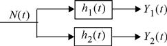
A white Gaussian noise process, N(t), is input to two filters with impulse responses, h1(t) and h2(t), as shown in the accompanying figure. The corresponding outputs are Y1(t) and Y2 (t), respectively.
(a) Derive an expression for the cross-correlation function of the two outputs, R Y1 Y2 (τ).
(b) Derive an expression for the cross-spectral density of the two outputs, S Y1 Y2 (τ).
(c) Under what conditions (on the filters) are the two outputs independent when sampled at the same instants in time? That is, when are Y1(to) and Y2(to) independent? Express your constraints in terms of the impulse responses of the filters and also in terms of their transfer functions.
(d) Under what conditions (on the filters) are the two outputs independent when sampled at different instants in time. That is, when are Y1 (t1) and Y2(t2) independent for arbitrary t1 and t2? Express your constraints in terms of the impulse responses of the filters and also in terms of their transfer functions.
11.13 If the inputs to two linear filters h1 (t) and h2(t) are X1 (t) and X2(t), respectively, show that the cross-correlation between the outputs Y1(t) and Y2 (t) of the two filters is
![]()
Section 11.2: Discrete-Time Systems
11.14 Is the following function a valid discrete-time autocorrelation function? Justify your answer.

11.15 A discrete random sequence X[n] is the input to a discrete linear filter h [n]. The output is Y[n]. Let Z[n] = X[n + i] − Y[n]. Find E[Z2[n]] in terms of the autocorrelation functions for X[n] and Y[n] and the cross-correlation function between X[n] and Y[n].
11.16 The unit impulse response of a discrete linear filter is h[n] = anu[n], where |a| ≤ 1. The autocorrelation function for the input random sequence is

Determine the cross-correlation function between the input and output random sequences.
11.17 Find the PSD of a discrete random sequence with the following autocorrelation function: RXX [k] = a(bk ), where |b| ≤ 1.
11.18 A discrete-time linear filter has a unit pulse response h [n]. The input to this filter is a random sequence with uncorrelated samples. Show that the output PSD is real and non-negative.
11.19 The input, X[k], to a filter is a discrete-time zero-mean random process whose autocorrelation function is RXX
[n] δ[n]. The input/output relationship of the filter is given by
11.20 The input to a filter is a discrete-time, zero-mean, random process whose autocorrelation function is
![]()
for some constant a such that |a| ≤ 1. We wish to filter this process so that the output of the filter is white. That is, we want the output, Y[k], to have an autocorrelation function, RYY [n] = δ[n].
Section 11.3: Noise Equivalent Bandwidth
11.21 Determine the noise equivalent bandwidth for a filter with impulse response
![]()
11.22 A filter has the following transfer function:
![]()
Determine the ratio of the noise equivalent bandwidth for this filter to its 3-dB bandwidth.
11.23 Suppose you want to learn the characteristics of a certain filter. A white noise source with an amplitude of 15 watts/Hz is connected to the input of the filter. The power spectrum of the filter output is measured and found to be
![]()
(a) What is the bandwidth (3 dB) of the filter?
(b) What is the attenuation (or gain) at zero frequency?
(c) Show one possible (i.e., real, causal) filter that could have produced this output PSD.
11.24 A filter has an impulse response of h(t) = te−t u(t). Find the noise equivalent bandwidth of the filter.
11.25 A filter has a transfer function given by
![]()
11.26 The definition for the noise equivalent bandwidth of a filter was given in terms of the transfer function of the filter in Definition 11.1. Derive an equivalent expression for the noise equivalent bandwidth of a filter in terms of the impulse response of the filter, h (t).
11.27 Suppose a filter has a transfer function given by H(f) = sine2(f). Find the noise equivalent bandwidth of the filter. Hint: You might want to use the result of Exercise 11.26.
Section 11.4: Signal-to-Noise Ratios

11.28 For the high-pass RC network shown, let X(t) = A sin (ωct + Θ) + N(t), where N(t) is white, WSS, Gaussian noise and Θ is a random variable uniformly distributed over [0, 2 π). Assuming zero initial conditions:
(a) Find the output mean and variance.
(b) Find and plot the autocorrelation function of the output.
11.29 A parallel RLC network is driven by an input current source of X(t) = A sin(ωc t + Θ) + N(t), where N(t) is white, WSS noise with zero-mean. The output is the voltage across the network. The phase Θ is a random variable uniformly distributed over [0, 2π).
(a) Find the output power spectrum by first computing the output autocorrelation function and then transforming.
(b) Check the result of part (a) by using (11.12c).
(c) Determine the output SNR and optimize the bandwidth to maximize the SNR. Assume ωc differs from the center frequency of the RLC filter.
Hints: You may have to calculate the autocorrelation function as a function of t and τ and then let t go to infinity to find the steady-state output. There are several conditions you may want to consider; for example, the filter may be overdamped, critically damped, or under damped. It may also have an initial voltage on the capacitor and a current through the inductor. State your assumption about these conditions.
11.30 A one-sided exponential pulse, s (t) = exp (−t)u (t), plus white noise is input to the finite time integrator of Exercise 11.1. Adjust the width of the integrator, to , so that the output SNR is maximized at t = to .
11.31 A square pulse of width to = 1 μs plus zero-mean white Gaussian noise is input to a filter with impulse response, h(t) = exp (−t/ti)u(t).
(a) Find the value of the constant t1 such that the SNR at the output of the filter will be maximum.
(b) Assuming the square pulse is non-zero over the time interval (0, to ), at what sampling time will the SNR at the output of the filter be maximized?
11.32 The input to a filter consists of a half-sinusoidal pulse

plus zero-mean white Gaussian noise.
(a) Suppose the impulse response of the filter is rectangular, h (t) = rect(t/ta). What should the width of the rectangle, ta, be in order to maximize the SNR at the output? At what point in time does that maximum occur?
(b) Suppose the impulse response of the filter is triangular, h (t) = tri (t/tb). What should the width of the triangle, tb, be in order to maximize the SNR at the output? At what point in time does that maximum occur?
(c) Which filter (rectangle or triangle) produces the larger SNR and by how much? Specify your answer in decibels (dBs).
Section 11.5: The Matched Filter
(a) Determine the impulse response of the filter matched to the pulse shape shown in the accompanying figure. Assume that the filter is designed to maximize the output SNR at time t = 3to.

(b) Sketch the output of the matched filter designed in part (a) when the signal s (t) is at the input.
11.34 Find the impulse response and transfer function of a filter matched to a triangular waveform as shown in the accompanying figure when the noise is stationary and white with a power spectrum of No/2.

11.35 A known deterministic signal, s (t), plus colored (not white) noise, N(t), with a PSD of SNN(f) is input to a filter. Derive the form of the filter that maximizes the SNR at the output of the filter at time t = to. To make this problem simpler, you do not need to insist that the filter is causal.
11.36 Consider the system described in Example 11.6 where a communication system transmits a square pulse of width t1. In that example, it was found that the matched filter can be implemented as a finite time integrator which integrates over a time duration to t1 seconds. For the sake of this problem, suppose t1 = 100 μs. Suppose that due to imperfections in the construction of this filter, we actually implement a filter which integrates over a time interval of t2 seconds. Determine what range of values of t2 would produce an output SNR which is within 0.25 dB of the optimal value (when t2 = tx). The answer to this question will give you an idea of how precise the design of the match filter needs to be (or how impercise it can be).
Section 11.6: The Wiener Filter
11.37 Suppose we observe a random process Z(t) (without any noise) over a time interval (−∞, t). Based on this observation, we wish to predict the value of the same random process at time t + to. That is, we desire to design a filter with impulse response, h (t), whose output will be an estimate of Z(t + to):
![]()
(a) Find the Wiener−Hopf equation for the optimum (in the minimum mean square error (MMSE) sense) filter.
(b) Find the form of the Wiener filter if RZZ(τ) = exp(−|τ|).
(c) Find an expression for the mean square error E[ε2(t)] = E[(Z(t + to) − Y(t))2].
11.38 Suppose we are allowed to observe a random process Z(t) at two points in time, to and t2. Based on those observations we would like to estimate Z(t) at time t = t1 where t0≤t1 ≤t2. We can view this as an interpolation problem. Let our estimator be a linear combination of the two observations,
![]()
(a) Use the orthogonality principle to find the MMSE estimator.
(b) Find an expression for the mean square error of the MMSE estimator.
11.39 Suppose we are allowed to observe a random process Z(t) at two points in time, t0 and t1. Based on those observations we would like to estimate Z(t) at time t = t2 where t0 ≤ t1 ≤ t2. We can view this as a prediction problem. Let our estimator be a linear combination of the two observations,
![]()
(a) Use the orthogonality principle to find the MMSE estimator.
(b) Suppose that RZZ (τ) = cexp(−b|τ|) for positive constants b and c. Show that in this case, the sample at time t = t0 is not useful for predicting the value of the process at time t = t2 (given we have observed the process at time t = t1 > t0). In other words, show that a = 0.
11.40 The sum of two independent random processes with PSDs
![]()
are input to a LTI filter.
(a) Determine the Wiener smoothing filter. That is, find the impulse response of the filter that produces an output that is an MMSE estimate of S (t).
11.41 The sum of two independent random sequences with autocorrelation functions

is input to an LTI filter.
(a) Determine the Wiener smoothing filter. That is, find the impulse response of the filter which produces an output which is an MMSE estimate of S[n].
(b) Find the PSD of the filtered signal plus noise.
(c) Find the input SNR and an estimate of the output SNR. Discuss whether or not the Wiener filter improves the SNR.
Hint: Compare the spectra of the Wiener filter, the signal, and the noise by plotting each on the same graph.
Section 11.7: Narrowband Random Processes and Complex Envelopes
11.42 The PSD of a narrowband Gaussian noise process, N(t), is as shown in the accompanying figure.
(a) Find and sketch the PSD of the I and Q components of the narrowband noise process.

(b) Find and sketch the cross-spectral density of the I and Q components.
11.43 The narrowband noise process of Exercise 11.42 is passed through the system shown in the accompanying figure. In the system, the LPF has a bandwidth which is large compared to B but small compared to fo.
(a) Show that the output of the system is proportional to |Gn(t)|2, where Gn(t) is the complex envelope of N(t).
(b) Find and sketch the autocorrelation function of the output of the system. (Hint: You might find the Gaussian moment factoring theorem useful, see Exercise 6.18.)
11.44 Let Z(t) be a zero-mean, stationary, narrowband process whose I and Q components are X(t) and Y(t), respectively. Show that the complex envelope,
![]()
MATLAB Exercises
(a) Construct a signal plus noise random sequence using 10 samples of
![]()
where N[n] is generated using randn in MATLAB and fo = 0.1/ts. Design a discrete-time matched filter for the cosine signal. Filter the signal plus noise sequence with the matched filter. At what sample value does the filter output peak.
(b) Construct a signal plus noise random sequence using 10 samples of the following
![]()
where N[n] is generated using randn in MATLAB, f1= 0.1/ts, and f2= 0.4/ts. Design a discrete-time matched filter for the f2 cosine signal. Filter the signal plus noise sequence with the matched filter. At what sample value does the filter output peak.
11.46 If a random sequence has an autocorrelation function Rxx[k] = 10(0.8|k|), find the discrete-time, pure prediction Wiener filter. That is, find the filter h [n] such that when X[n] is input the output, Y[n], will be an MMSE estimate of X[n +1]. Determine and plot the PSD for the random sequence and the power transfer function, |H(f)|2, of the filter.
11.47 You have a random process with the following correlation matrix,

Determine the pure prediction Wiener filter. That is, find the coefficients of the impulse response, h = [h0, h1, h2, 0, 0, 0, …]. Then determine the power spectrum of the Wiener filter. Are the results what you expected?
11.48 Generate a 100-point random sequence using randn(1,100) in MATLAB. Use a first-order AR filter to filter this random process. That is, the filter is
![]()
Let a1 = −0.1. Use the filtered data to obtain an estimate for the first-order prediction Wiener filter. Compare the estimated filter coefficient with the true value.
1 The notation x(t) infin y (t) means that x(t) is proportional to y (t).
2 The same disclaimer must be made here as in Definition 5.13. Many texts do not include the factor of 1/2 in the definition of the autocorrelation function for complex random processes, and therefore the reader should be aware that there are two different definitions prevalent in the literature.