
CHAPTER 4
Operations on a Single Random Variable
In our study of random variables, we use the probability density function (PDF), the cumulative distribution function (CDF), or the probability mass function (PMF) to provide a complete statistical description of the random variable. From these functions, we could, in theory, determine just about anything we might want to know about the random variable. In many cases, it is of interest to distill this information down to a few parameters which describe some of the important features of the random variable. For example, we saw in Chapter 3 that the Gaussian random variable is described by two parameters, which were referred to as the mean and variance. In this chapter, we look at these parameters as well as several others that describe various characteristics of random variables. We see that these parameters can be viewed as the results of performing various operations on a random variable.
4.1 Expected Value of a Random Variable
To begin, we introduce the idea of an average or expected value of a random variable. This is perhaps the single most important characteristic of a random variable and also is a concept that is very familiar to most students. After taking a test, one of the most common questions a student will ask after they see their grade is “What was the average?” On the other hand, how often does a student ask “What was the PDF of the exam scores?” While the answer to the second question would provide the student with more information about how the class performed, the student may not want all that information. Just knowing the average may be sufficient to tell the student how he/she performed relative to the rest of the class.
Definition 4.1: The expected value of a random variable X which has a PDF, fX(x), is
![]() (4.1)
(4.1)
The terms average, mean, expectation, and first moment are all alternative names for the concept of expected value and will be used interchangeably throughout the text. Furthermore, an overbar is often used to denote expected value so that the symbol ![]() is to be interpreted as meaning the same thing as E[X]. Another commonly used notation is to write μX = E[X].
is to be interpreted as meaning the same thing as E[X]. Another commonly used notation is to write μX = E[X].
For discrete random variables, the PDF can be written in terms of the PMF,
![]() (4.2)
(4.2)
In that case, using the properties of delta functions, the definition of expected values for discrete random variables reduces to
![]() (4.3)
(4.3)
Hence, the expected value of a discrete random variable is simply a weighted average of the values that the random variable can take on, weighted by the probability mass of each value. Naturally, the expected value of a random variable only exists if the integral in Equation (4.1) or the series in Equation (4.3) converges. One can dream up many random variables for which the integral or series does not converge and hence their expected values don’t exist (or less formally, their expected value is infinite). To gain some physical insight into this concept of expected value, we may think of fX(x) as a mass distribution of an object along the x axis, then Equation (4.1) calculates the centroid or center of gravity of the mass.
Example 4.1
Consider a random variable that has an exponential PDF given by ![]() . Its expected value is calculated as follows:
. Its expected value is calculated as follows:
![]()
The last equality in the series is obtained by using integration by parts once. It is seen from this example that the parameter b which appears in this exponential distribution is in fact the mean (or expected value) of the random variable.
Example 4.2
Next, consider a Poisson random variable whose PMF is given by ![]() . Its expected value is found in a similar manner.
. Its expected value is found in a similar manner.
![]()
Once again, we see that the parameter a in the Poisson distribution is equal to the mean.
Example 4.3
In the last two examples, we saw random variables whose PDF or PMF was described by a single parameter which in both cases turned out to be the mean. We work one more example here to show that this does not always have to be the case. Consider a Rayleigh random variable with PDF
![]()
The mean is calculated as follows:
![]()
The last equality is obtained using the fact that ![]() . Alternatively (for those students not familiar with the properties of Γ functions), one could obtain this result using integration by parts once on the original integral (setting u = x and dv = (x/σ2)exp(−x2/(2σ2))). In this case, neither the parameter σ nor σ2 is equal to the expected value of the random variable. However, since the mean is proportional to σ, we could, if we wanted to, rewrite the Rayleigh PDF in terms of its expected value, μX, as follows:
. Alternatively (for those students not familiar with the properties of Γ functions), one could obtain this result using integration by parts once on the original integral (setting u = x and dv = (x/σ2)exp(−x2/(2σ2))). In this case, neither the parameter σ nor σ2 is equal to the expected value of the random variable. However, since the mean is proportional to σ, we could, if we wanted to, rewrite the Rayleigh PDF in terms of its expected value, μX, as follows:
![]()
4.2 Expected Values of Functions of Random Variables
The concept of expectation can be applied to the functions of random variables as well as to the random variable itself. This will allow us to define many other parameters that describe various aspects of a random variable.
Definition 4.2: Given a random variable X with PDF fX(x), the expected value of a function, g(X), of that random variable is given by
![]() (4.4)
(4.4)
For a discrete random variable, this definition reduces to
![]() (4.5)
(4.5)
To start with, we demonstrate one extremely useful property of expectations in the following theorem.
Theorem 4.1: For any constants a and b,
![]() (4.6)
(4.6)
Furthermore, for any function g(x) which can be written as a sum of several other functions (i.e., g(x) = g1(x) + g2(x) + … + gN(x)),
 (4.7)
(4.7)
In other words, expectation is a linear operation and the expectation operator can be exchanged (in order) with any other linear operation.
Proof: The proof follows directly from the linearity of the integration operator.
 (4.8)
(4.8)
The second part of the theorem is proved in an identical manner:
 (4.9)
(4.9)
Different functional forms of g(X) lead to various different parameters which describe the random variable and are known by special names. A few of the more common ones are listed in Table 4.1. In the following sections, selected parameters will be studied in more detail.
Table 4.1. Expected values of various functions of random variables
| Name | Function of X | Expected Value, Notation |
| Mean, average, expected value, expectation, first moment | g(x) =x | |
| nth moment | g(x) =xn | |
| nth central moment | g(x) = (x –μX)n | |
| Variance | g(x) = (x –μX)2 | |
| Coefficient of skewness |  |
 |
| Coefficient of kurtosis |  |
 |
| Characteristic function | g(x) = ejωx | ΦX(ω) = E[ejωX] |
| Moment-generating function | g(x) = esx | MX(s) =E [esX] |
| Probability-generating function | g(x) =zx | HX(z) =E [zX] |
4.3 Moments
Definition 4.3: The nth moment of a random variable X is defined as
![]() (4.10)
(4.10)
For a discrete random variable, this definition reduces to
![]() (4.11)
(4.11)
The zeroth moment is simply the area under the PDF and must be one for any random variable. The most commonly used moments are the first and second moments. The first moment is what we previously referred to as the mean, while the second moment is the mean-squared value. For some random variables, the second moment might be a more meaningful characterization than the first. For example, suppose X is a sample of a noise waveform. We might expect that the distribution of the noise is symmetric about zero (i.e., just as likely to be positive as negative) and hence the first moment will be zero. So if we are told that X has a zero mean, all this says is merely that the noise does not have a bias. However, the second moment of the random noise sample is in some sense a measure of the strength of the noise. In fact, in Chapter 10, we will associate the second moment of a noise process with the power in the process. Thus, specifying the second moment can give us some useful physical insight into the noise process.
Example 4.4
Consider a discrete random variable that has a binomial distribution. Its probability mass function is given by
![]()
The first moment is calculated as follows:

In this last expression, the summand is a valid PMF (i.e., that of a binomial random variable with parameters p and n – 1) and therfore must sum to unity. Thus, E[X] = np. To calculate the second moment, we employ a helpful little trick. Note that we can write k2 = k(k − 1) + k. Then
![]()
The second sum is simply the first moment, which has already been calculated. The first sum is evaluated in a manner similar to that used to calculate the mean.
![]()
![]()
![]()
Putting these two results together gives
![]()
Example 4.5
Consider a random variable with a uniform PDF given as
![]()
The mean is given by
![]()
while the second moment is
![]()
In fact, it is not hard to see that in general, the n th moment of this uniform random variable is given by
![]()
4.4 Central Moments
Consider a random variable Y which could be expressed as the sum, Y = a + X of a deterministic (i.e., not random) part a and a random part X. Furthermore, suppose that the random part tends to be very small compared to the fixed part. That is, the random variable Y tends to take small fluctuations about a constant value, a. Such might be the case in a situation where there is a fixed signal corrupted by noise. In this case, we might write Yn = (a + X)n ≈ an. As such, the nth moment of Y would be dominated by the fixed part. That is, it is difficult to characterize the randomness in Y by looking at the moments. To overcome this, we can use the concept of central moments.
Definition 4.4: The n th central moment of a random variable X is defined as
![]() (4.12)
(4.12)
In the above equation, μX is the mean (first moment) of the random variable. For discrete random variables, this definition reduces to
![]() (4.13)
(4.13)
With central moments, the mean is subtracted from the variable before the moment is taken in order to remove the bias in the higher moments due to the mean. Note that, like regular moments, the zeroth central moment is E[(X − μX)0] = E[1] = 1. Furthermore, the first central moment is E[X − μX] = E[X] − μX = μX − μX = 0. Hence, the lowest central moment of any real interest is the second central moment. This central moment is given a special name, the variance, and we quite often use the notation σX2 to represent the variance of the random variable X. Note that
 (4.14)
In many cases, the best way to calculate the variance of a random variable is to calculate the first two moments and then form the second moment minus the first moment squared.
Example 4.6
For the binomial random variable in Example 4.4, recall that the mean was E[X] = np and the second moment was E[X2] = n2p2 + np(1 − p). Therefore, the variance is given by σX2 = np(1 − p). Similarly, for the uniform random variable in Example 4.5, E[X] = a/2, E[X2] = a2/3, and therfore σ2X = a2/3−a2/4 = a2/12. Note that if the moments have not previously been calculated, it may be just as easy to compute the variance directly. In the case of the uniform random variable, once the mean has been calculated, the variance can be found as

Another common quantity related to the second central moment of a random variable is the standard deviation, which is defined as the square root of the variance,
![]() (4.15)
(4.15)
Both the variance and the standard deviation serve as a measure of the width of the PDF of a random variable. Some of the higher-order central moments also have special names, although they are much less frequently used. The third central moment is known as the skewness and is a measure of the symmetry of the PDF about the mean. The fourth central moment is called the kurtosis and is a measure of the peakedness of a random variable near the mean. Note that not all random variables have finite moments and/or central moments. We give an example of this later for the Cauchy random variable. Some quantities related to these higher-order central moments are given in the following definition.
Definition 4.5: The coefficient of skewness is
 (4.16)
This is a dimensionless quantity that is positive if the random variable has a PDF skewed to the right and negative if skewed to the left. The coefficient of kurtosis is also dimensionless and is given as
 (4.17)
The more the PDF is concentrated near its mean, the larger the coefficient of kurtosis. In other words, a random variable with a large coefficient of kurtosis will have a large peak near the mean.
Example 4.7
An exponential random variable has a PDF given by
![]()
The mean value of this random variable is μX = 1/b. The nth central moment is given by
In the preceding expression, it is understood that 0! = 1. As expected, it is easily verified from the above expression that the 0th central moment is 1 and the first central moment is 0. Beyond these, the second central moment is σX2 = 1/b2, the third central moment is E[(X − 1/b)3] = −2/b3, and the fourth central moment is E[(X − 1/b)4] = 9/b4. The coefficients of skewness and kurtosis are given by
The fact that the coefficient of skewness is negative shows that the exponential PDF is skewed to the left of its mean.
Example 4.8
Next consider a Laplace (two-sided exponential) random variable with a PDF given by
![]()
Since this PDF is symmetric about zero, its mean is zero and therefore in this case the central moments are simply the moments,
![]()
Since the two-sided exponential is an even function and xn is an odd function for any odd n, the integrand is then an odd function for any odd n. The integral of any odd function over an interval symmetric about zero is equal to zero, and hence all odd moments of the Laplace random variable are zero. The even moments can be calculated individually:
The coefficient of skewness is zero (since the third central moment is zero) and the coefficient of kurtosis is
![]()
Note that the Laplace distribution has a sharp peak near its mean as evidenced by a large coefficient of kurtois. The fact that the coefficient of skewness is zero is consistent with the fact that the distribution is symmetric about its mean.
Example 4.9
 It is often the case that the PDF of random variables of practical interest may be too complicated to allow us to compute various moments and other important parameters of the distribution in an analytic fashion. In those cases, we can use a computer to calculate the needed quantities numerically. Take for example a Rician random variable whose PDF is given by
![]()
Suppose we wanted to know the mean of this random variable. This requires us to evaluate
![]()
Note that the parameter σ2 which shows up in the Rician PDF is not the variance of the Rician random variable. While analytical evaluation of this integral looks formidable, given numerical values for a and σ2, this integral can be evaluated (at least approximately) using standard numerical integration techniques. In order to use the numerical integration routines built into MATLAB, we must first write a function which evaluates the integrand. For evaluating the mean of the Rician PDF, this can be accomplished as follows (see Appendix D, Equation (D.52) for an analytic expression for the mean):

Once this function is defined, the MATLAB function quads can be called upon to perform the numerical integration. For example, if a = 2 and σ = 3, the mean could be calculated as follows:
![]()
Executing this code produced an answer of μX = 4.1665. Note that in order to calculate the mean, the upper limit of the integral should be infinite. However using limit2=Inf in the above code would have led MATLAB to produce a result of NaN (“not a number”). Instead, we must use an upper limit sufficiently large that for the purposes of evaluating the integral it is essentially infinite. This can be done by observing the integrand and seeing at what point the integrand dies off. The reader is encouraged to execute the code in this example using different values of the upper integration limit to see how large the upper limit must be to produce accurate results.
4.5 Conditional Expected Values
Another important concept involving expectation is that of conditional expected value. As specified in Definition 4.6, the conditional expected value of a random variable is a weighted average of the values the random variable can take on, weighted by the conditional PDF of the random variable.
Definition 4.6: The expected value of a random variable X, conditioned on some event A is
![]() (4.18)
(4.18)
For a discrete random variable, this definition reduces to
![]() (4.19)
(4.19)
Similarly, the conditional expectation of a function, g(·), of a random variable, conditioned on the event A is
 (4.20)
depending on whether the random variable is continuous or discrete.
Conditional expected values are computed in the same manner as regular expected values with the PDF or PMF replaced by a conditional PDF or conditional PMF.
Example 4.10
Consider a Gaussian random variable of the form
![]()
Suppose the event A is the event that the random variable X is positive, A = {X>0}. Then
![]()
The conditional expected value of X given that X>0 is then
![]()
4.6 Transformations of Random Variables
Consider a random variable X with a PDF and CDF given by fX(x) and FX(x), respectively. Define a new random variable Y such that Y = g(X) for some function g(·). What is the PDF, fY(y), (or CDF) of the new random variable? This problem is often encountered in the study of systems where the PDF for the input random variable X is known and the PDF for the output random variable Y needs to be determined. In such a case, we say that the input random variable has undergone a transformation.
4.6.1 Monotonically Increasing Functions
To begin our exploration of transformations of random variables, let us assume that the function is continuous, one-to-one, and monotonically increasing. A typical function of this form is illustrated in Figure 4.1a. This assumption will be lifted later when more general functions are considered, but for now this simpler case applies. Under these assumptions, the inverse function, X = g−1 (Y), exists and is well behaved. In order to obtain the PDF of Y, we first calculate the CDF. Recall that FY(y) = Pr(Y ≤ y). Since there is a one-to-one relationship between values of Y and their corresponding values of X, this CDF can be written in terms of X according to
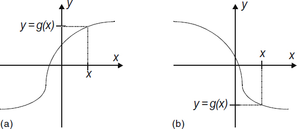
Figure 4.1 (a) A monotonic increasing function and (b) a monotonic decreasing function.
![]() (4.21)
(4.21)
Note, this can also be written as
![]() (4.22)
(4.22)
Differentiating Equation (4.21) with respect to y produces
 (4.23)
while differentiating Equation (4.22) with respect to x gives
 (4.24)
Either Equation (4.23) or (4.24) can be used (whichever is more convenient) to compute the PDF of the new random variable.
Example 4.11
Suppose X is a Gaussian random variable with mean, μ, and variance, σ2. A new random variable is formed according to Y= aX + b, where a > 0 (so that the transformation is monotonically increasing). Since dy/dx = a, then applying Equation (4.24) produces
![]()
Furthermore, plugging in the Gaussian PDF of X results in

Note that the PDF of Y still has a Gaussian form. In this example, the transformation did not change the form of the PDF; it merely changed the mean and variance.
Example 4.12
Let X be an exponential random variable with fX{x) = 2e−2x u(x) and let the transformation be Y = X3. Then dy/dx = 3x2 and

Example 4.13
Suppose a phase angle Θ is uniformly distributed over (−π/2, π2) and the transformation is Y = sin(Θ). Note that in general y = sin(θ) is not a monotonic transformation, but under the restriction −π/2 ≤ θ ≤ π2, this transformation is indeed monotonically increasing. Also note that with this transformation the resulting random variable, Y, must take on values in the range (−1, 1). Therefore, whatever PDF is obtained for Y, it must be understood that the PDF is zero outside (−1, 1). Applying Equation (4.24) gives
![]()
This is known as an arcsine distribution.
4.6.2 Monotonically Decreasing Functions
If the transformation is monotonically decreasing rather than increasing, a simple modification to the previous derivations can lead to a similar result. First, note that for monotonic decreasing functions, the event {Y ≤ y} is equivalent to the event X ≥ g−1 (y), giving us
![]() (4.25)
(4.25)
Differentiating with respect to y gives
 (4.26)
Similarly, writing FY(g(x)) = 1 − FX(x) and differentiating with respect to x results in
 (4.27)
Equations (4.23), (4.24), (4.26), and (4.27) can be consolidated into the following compact form:
 (4.28)
where now the sign differences have been accounted for by the absolute value operation. This equation is valid for any monotonic function, either monotonic increasing or monotonic decreasing.
4.6.3 Nonmonotonic Functions
Finally, we consider a general function which is not necessarily monotonic. Figure 4.2 illustrates one such example. In this case, we cannot associate the event {Y ≤ y} with events of the form {X ≤ g−1 (y)} or {X ≥ g−1 (y)} because the transformation is not monotonic. To avoid this problem, we calculate the PDF of Y directly, rather than first finding the CDF. Consider an event of the form {y ≤ Y ≤ y + dy] for an infinitesimal dy. The probability of this event is Pr(y ≤ Y ≤ y + dy) = fY(y)dy. In order to relate the PDF of Y to the PDF of X, we relate the event {y ≤ Y ≤ y + dy} to events involving the random variable X. Because the transformation is not monotonic, there may be several values of x which map to the same value of y. These are the roots of the equation x = g−1 (y). Let us refer to these roots as x1, x2, …, xN. Furthermore, let X+ be the subset of these roots at which the function g(x) has a positive slope and similarly let X− be the remaining roots for which the slope of the function is negative. Then

Figure 4.2 A nonmonotonic function; the inverse function may have multiple roots.
 (4.29)
Since each of the events on the right-hand side is mutually exclusive, the probability of the union is simply the sum of the probabilities so that
 (4.30)
Again, invoking absolute value signs to circumvent the need to have two separate sums and dividing by dy, the following result is obtained:
 (4.31)
When it is more convenient, the equivalent expression
 (4.32)
can also be used. The following theorem summarizes the general formula for transformations of random variables.
Theorem 4.2: Given a random variable X with known PDF, fX(x), and a transformation Y = g(X). The PDF of Y is
 (4.33)
where the xi are the roots of the equation y = g(x). The proof precedes the theorem.
Example 4.14
Suppose X is a Gaussian random variable with zero mean and variance σ2 together with a quadratic transformation, Y = X2. For any positive value of y, y = x2 has two real roots, namely ![]() (for negative values of y there are no real roots). Application of Equation (4.33) gives
(for negative values of y there are no real roots). Application of Equation (4.33) gives
![]()
For a zero-mean Gaussian PDF, fX(x) is an even function so that ![]() . Therefore,
. Therefore,
![]()
Hence, Y is a Gamma random variable.
Example 4.15
Suppose the same Gaussian random variable from the previous example is passed through a half-wave rectifier which is described by the input-output relationship
![]()
For x > 0, dy/dx = 1 so that fY(y) = fX(y). However, when x ≤ 0, dy/dx = 0, which will create a problem if we try to insert this directly into Equation (4.33). To treat this case, we note that the event X ≤ 0 is equivalent to the event Y=0; therefore, Pr(Y = 0) = Pr(X ≤ 0). Since the input Gaussian PDF is symmetric about zero, Pr(X ≤ 0) = 1/2. Basically, the random variable Y is a mixed random variable. It has a continuous part over the region y>0 and a discrete part at y = 0. Using a delta function, we can write the PDF of Y as
![]()
Example 4.15 illustrates how to deal with transformations that are flat over some interval of nonzero length. In general, suppose the transformation y = g(x) is such that g(x) = yo for any x in the interval x1 ≤ x ≤ x2. Then the PDF of Y will include a discrete component (a delta function) of height Pr(Y=yo) = Pr(x1 ≤ x ≤ x2) at the point y = y. One often encounters transformations that have several different flat regions. One such “staircase” function is shown in Figure 4.3. Hence, a random variable X that may be continuous will be converted into a discrete random variable. The classical example of this is analog-to-digital conversion of signals. Suppose the transformation is of a general staircase form,

Figure 4.3 A staircase (quantizer) transformation: a continuous random variable will be converted into a discrete random variable.
 (4.34)
Then Y will be a discrete random variable whose PMF is
 (4.35)
Example 4.16
Suppose X is an exponential random variable with a PDF fX(x) = exp(−x)u(x) and we form a new random variable Y by rounding X down to the nearest integer. That is,
![]()
Then, the PMF of Y is
![]()
Hence, quantization of an exponential random variable produces a geometric random variable.
Example 4.17
Let X be a random variable uniformly distributed over (−a/2, a/2). Accordingly, its PDF is of the form
![]()
A new random variable is to be formed according to the square law transformation Y = X2. Applying the theory developed in this section you should be able to demonstrate that the new random variable has a PDF given by
![]()
Using MATLAB, we create a large number of samples of the uniform random variable, pass these samples through the square law transformation, and then construct a histogram of the resulting probability densities. The MATLAB code to do so follows and the results of running this code are shown in Figure 4.4.
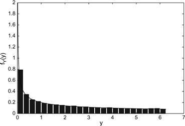
Figure 4.4 Comparison of estimated and true PDF for Example 4.17. (For color version of this figure, the reader is refered to the web version of this chapter).

4.7 Characteristic Functions
In this section, we introduce the concept of a characteristic function. The characteristic function of a random variable is closely related to the Fourier transform of the PDF of that random variable. Thus, the characteristic function provides a sort of “frequency domain” representation of a random variable, although in this context there is no connection between our frequency variable ω and any physical frequency. In studies of deterministic signals, it was found that the use of Fourier transforms greatly simplified many problems, especially those involving convolutions. We will see in future chapters the need for performing convolution operations on PDFs of random variables, and hence frequency domain tools will become quite useful. Furthermore, we will find that characteristic functions have many other uses. For example, the characteristic function is quite useful for finding moments of a random variable. In addition to the characteristic function, two other related functions, namely, the moment-generating function (analogous to the Laplace transform) and the probability-generating function (analogous to the z-transform), will also be studied in the following sections.
Definition 4.7: The characteristic function of a random variable, X, is given by
![]() (4.36)
(4.36)
Note the similarity between this integral and the Fourier transform. In most of the electrical engineering literature, the Fourier transform of the function fX(x) would be Φ(−ω). Given this relationship between the PDF and the characteristic function, it should be clear that one can get the PDF of a random variable from its characteristic function through an inverse Fourier transform operation:
![]() (4.37)
(4.37)
The characteristic functions associated with various random variables can be easily found using tables of commonly used Fourier transforms, but one must be careful since the Fourier integral used in Equation (4.36) may be different from the definition used to generate common tables of Fourier transforms. In addition, various properties of Fourier transforms can also be used to help calculate characteristic functions as shown in the following example.
Example 4.18
An exponential random variable has a PDF given by fX(x) = exp(−x)u(x). Its characteristic function is found to be
![]()
This result assumes that ω is a real quantity. Now suppose another random variable Y has a PDF given by fY(y) = a exp(−ay)u(y). Note that fY(y) = afX(ay), thus using the scaling property of Fourier transforms, the characteristic function associated with the random variable Y is given by
![]()
assuming a is a positive constant (which it must be for Y to have a valid PDF). Finally, suppose that Z has a PDF given by fZ(z) = a exp(−a(z − b))u(z − b). Since fZ(z) = fY(z − b), the shifting property of Fourier transforms can be used to help find the characteristic function associated with the random variable Z:
![]()
The next example demonstrates that the characteristic function can also be computed for discrete random variables. In Section 4.8, the probability-generating function will be introduced which is preferred by some when dealing with discrete random variables.
Example 4.19
A binomial random variable has a PDF which can be expressed as
![]()
Its characteristic function is computed as follows:

Since the Gaussian random variable plays such an important role in so many studies, we derive its characteristic function in Example 4.20. We recommend that the student commit the result of this example to memory. The techniques used to arrive at this result are also important and should be carefully understood.
Example 4.20
For a standard normal random variable, the characteristic function can be found as follows:
![]()
To evaluate this integral, we complete the square in the exponent.
![]()
The integrand in the above expression looks like the properly normalized PDF of a Gaussian random variable, and since the integral is over all values of x, the integral must be unity. However, close examination of the integrand reveals that the “mean” of this Gaussian integrand is complex. It is left to the student to rigorously verify that this integral still evaluates to unity even though the integrand is not truly a Gaussian PDF (since it is a complex function and hence not a PDF at all). The resulting characteristic function is then
![]()
For a Gaussian random variable whose mean is not zero or whose standard deviation is not unity (or both), the shifting and scaling properties of Fourier transforms can be used to show that

Theorem 4.3: For any random variable whose characteristic function is differentiable at ω= 0,
![]() (4.38)
(4.38)
Proof: The proof follows directly from the fact that the expectation and differentiation operations are both linear and consequently the order of these operations can be exchanged.
![]()
Multiplying both sides by −j and evaluating at ω = 0 produces the desired result.
Theorem 4.3 demonstrates a very powerful use of the characteristic function. Once the characteristic function of a random variable has been found, it is generally a very straightforward thing to produce the mean of the random variable. Furthermore, by taking the kth derivative of the characteristic function and evaluating at ω = 0, an expression proportional to the kth moment of the random variable is produced. In particular,
 (4.39)
Hence, the characteristic function represents a convenient tool to easily determine the moments of a random variable.
Example 4.21
Consider the exponential random variable of Example 4.18 where fY(y) = a exp(−ay)u(y). The characteristic function was found to be
![]()
The derivative of the characteristic function is
![]()
and thus the first moment of Y is
![]()
For this example, it is not difficult to show that the kth derivative of the characteristic function is
![]()
and from this, the kth moment of the random variable is found to be
![]()
For random variables that have a more complicated characteristic function, evaluating the kth derivative in general may not be an easy task. However, Equation (4.39) only calls for the kth derivative evaluated at a single point (ω = 0), which can be extracted from the Taylor series expansion of the characteristic function. To see this, note that from Taylor’s theorem, the characteristic function can be expanded in a power series as
 (4.40)
If one can obtain a power series expansion of the characteristic function, then the required derivatives are proportional to the coefficients of the power series. Specifically, suppose an expansion of the form
 (4.41)
is obtained. Then the derivatives of the characteristic function are given by
 (4.42)
The moments of the random variable are then given by
![]() (4.43)
(4.43)
This procedure is illustrated using a Gaussian random variable in the next example.
Example 4.22
Consider a Gaussian random variable with a mean of μ = 0 and variance σ2. Using the result of Example 4.20, the characteristic function is ΦX(ω) = exp(−ω2σ2/2). Using the well-known Taylor series expansion of the exponential function, the characteristic function is expressed as
![]()
The coefficients of the general power series as expressed in Equation (4.41) are given by

Hence, the moments of the zero-mean Gaussian random variable are

As expected, E[X0] = 1, E[X] = 0 (since it was specified that μ = 0), and E[X2] = σ2 (since in the case of zero-mean variables, the second moment and variance are one and the same). Now, we also see that E[X3] = 0 (as are all odd moments), E[X4] = 3σ4, E[X6] = 15σ6, and so on. We can also conclude from this that for Gaussian random variables, the coefficient of skewness is cs = 0 while the coefficient of kurtosis is ck = 3.
In many cases of interest, the characteristic function has an exponential form. The Gaussian random variable is a typical example. In such cases, it is convenient to deal with the natural logarithm of the characteristic function.
Definition 4.8: In general, we can write a series expansion of ln[ΦX(ω)] as
 (4.44)
where the coefficients, λn, are called the cumulants and are given as
 (4.45)
The cumulants are related to the moments of the random variable. By taking the derivatives specified in Equation (4.45) we obtain
![]() (4.46)
(4.46)
![]() (4.47)
(4.47)
![]() (4.48)
(4.48)
Thus, λ1 is the mean, λ2 is the second central moment (or the variance), and λ3 is the third central moment. However, higher-order cumulants are not as simply related to the central moments.
4.8 Probability-Generating Functions
In the world of signal analysis, we often use Fourier transforms to describe continuous time signals, but when we deal with discrete time signals, it is common to use a z-transform instead. In the same way, the characteristic function is a useful tool for working with continuous random variables, but when discrete random variables are concerned, it is often more convenient to use a device similar to the z-transform which is known as the probability-generating function.
Definition 4.9: For a discrete random variable with a PMF, PX(k), defined on the nonnegative integers,1 k = 0, 1, 2, …, the probability-generating function, HX(z), is defined as
![]() (4.49)
(4.49)
Note the similarity between the probability-generating function and the unilateral z-transform of the PMF.
Since the PMF is seen as the coefficients of the Taylor series expansion of HX(z), it should be apparent that the PMF can be obtained from the probability-generating function through
 (4.50)
The derivatives of the probability-generating function evaluated at zero return the PMF and not the moments as with the characteristic function. However, the moments of the random variable can be obtained from the derivatives of the probability-generating function at z = 1.
Theorem 4.4: The mean of a discrete random variable can be found from its probability-generating function according to
![]() (4.51)
(4.51)
Furthermore, the higher-order derivatives of the probability-generating function evaluated at z = 1 lead to quantities which are known as the factorial moments,
 (4.52)
Proof: The result follows directly from differentiating Equation (4.49). The details are left to the reader.
It is a little unfortunate that these derivatives do not produce the moments directly, but the moments can be calculated from the factorial moments. For example,
 (4.53)
Hence, the second moment is simply the sum of the first two factorial moments. Furthermore, if we were interested in the variance as well, we would obtain
![]() (4.54)
(4.54)
Example 4.23
Consider the binomial random variable of Example 4.4 whose PMF is
![]()
The corresponding probability-generating function is
![]()
Evaluating the first few derivatives at z=1 produces

From these factorial moments, we calculate the mean, second moment, and variance of a binomial random variable as
![]()
In order to gain an appreciation for the power of these “frequency domain” tools, compare the amount of work used to calculate the mean and variance of the binomial random variable using the probability-generating function in Example 4.23 with the direct method used in Example 4.4.
As was the case with the characteristic function, we can compute higher-order factorial moments without having to take many derivatives, by expanding the probability-generating function into a Taylor series. In this case, the Taylor series must be about the point z = 1.
 (4.55)
Once this series is obtained, one can easily identify all of the factorial moments. This is illustrated using a geometric random variable in Example 4.24.
Example 4.24
A geometric random variable has a PMF given by PX(k) = (1 − p)pk, k = 0, 1, 2, … The probability-generating function is found to be
![]()
In order to facilitate forming a Taylor series expansion of this function about the point z = 1, it is written explicitly as a function of z–1. From there, the power series expansion is fairly simple.

Comparing the coefficients of this series with the coefficients given in Equation (4.55) leads to immediate identification of the factorial moments,
![]()
4.9 Moment-Generating Functions
In many problems, the random quantities we are studying are often inherently nonnegative. Examples include the magnitude of a random signal, the time between arrivals of successive customers in a queueing system, or the number of points scored by your favorite football team. The resulting PDFs of these quantities are naturally one-sided. For such one-sided waveforms, it is common to use Laplace transforms as a frequency domain tool. The moment-generating function is the equivalent tool for studying random variables.
Definition 4.10: The moment-generating function, MX(u), of a nonnegative2 random variable, X, is
![]() (4.56)
(4.56)
Note the similarity between the moment-generating function and the Laplace transform of the PDF.
The PDF can in principle be retrieved from the moment-generating function through an operation similar to an inverse Laplace transform,
 (4.57)
Because the sign in the exponential term in the integral in Equation (4.56) is the opposite of the traditional Laplace transform, the contour of integration (the so-called Bromwich contour) in the integral specified in Equation (4.57) must now be placed to the left of all poles of the moment-generating function. As with the characteristic function, the moments of the random variable can be found from the derivatives of the moment-generating function (hence, its name) according to
 (4.58)
It is also noted that if the moment-generating function is expanded in a power series of the form
 (4.59)
then the moments of the random variable are given by E[Xk] = k!mk.
Example 4.25
Consider an Erlang random variable with a PDF of the form
![]()
The moment-generating function is calculated according to
![]()
To evaluate this function, we note that the integral looks like the Laplace transform of the function xn−1/(n−1)! evaluated at s = 1−u. Using standard tables of Laplace transforms (or using integration by parts several times) we get
![]()
The first two moments are then found as follows:

From this, we could also infer that the variance is σX2 = n(n+ 1)−n2 = n. If we wanted a general expression for the kth moment, it is not hard to see that
![]()
4.10 Evaluating Tail Probabilities
A common problem encountered in a variety of applications is the need to compute the probability that a random variable exceeds a threshold, Pr(X > xo). Alternatively we might want to know, Pr(|X − μX| > xo). These quantities are referred to as tail probabilities. That is, we are asking, what is the probability that the random variable takes on a value that is in the tail of the distribution? While this can be found directly from the CDF of the random variable, quite often, the CDF may be difficult or even impossible to find. In those cases, one can always resort to numerical integration of the PDF. However, this involves a numerical integration over a semi-infinite region, which in some cases may be problematic. Then, too, in some situations, we might not even have the PDF of the random variable, but rather the random variable may be described in some other fashion. For example, we may only know the mean, or the mean and variance, or the random variable may be described by one of the frequency domain functions discussed in the previous sections. Obviously, if we are only given partial information about the random variable, we would not expect to be able to perfectly evaluate the tail probabilities, but we can obtain bounds on these probabilities. In this section, we present several techniques for obtaining various bounds on tail probabilities based on different information about the random variable. We then conclude the section by showing how to exactly evaluate the tail probabilities directly from one of the frequency domain descriptions of the random variables.
Theorem 4.5 (Markov’s inequality): Suppose that X is a nonnegative random variable (i.e., one whose PDF is nonzero only over the range [0, ∞)). Then,
![]() (4.60)
(4.60)
Proof: For nonnegative random variables, the expected value is
 (4.61)
Dividing both sides by xo gives the desired result.
Markov’s inequality provides a bound on the tail probability. The bound requires only knowledge of the mean of the random variable. Because the bound uses such limited information, it has the potential of being very loose. In fact, if xo ≤ E[X], then the Markov inequality states that Pr(X≥ xo) is bounded by a number that is greater than 1. While this is true, in this case the Markov inequality gives us no useful information. Even in less extreme cases, the result can still be very loose as shown by the next example.
Example 4.26
Suppose the average life span of a person was 78 years. The probability of a human living to be 110 years would then be bounded by
![]()
Of course, we know that in fact very few people live to be 110 years old, and hence this bound is almost useless to us.
If we know more about the random variable than just its mean, we can obtain a more precise estimate of its tail probability. In Example 4.26, we know that the bound given by the Markov’s inequality is ridiculously loose because we know something about the variability of the human life span. The next result allows us to use the variance as well as the mean of a random variable to form a different bound on the tail probability.
Theorem 4.6 (Chebyshev’s inequality): Suppose that X is a random variable with mean, μX, and variance, σ2X. The probability that the random variable takes on a value that is removed from the mean by more than xo is given by
 (4.62)
Proof: Chebyshev’s inequality is a direct result of Markov’s inequality. Note that the event {|X − μX|≥ xo} is equivalent to the event {(X − μX)2 ≥ x2o}. Applying Markov’s inequality to the later event results in
 (4.63)
Chebyshev’s inequality gives a bound on the two-sided tail probability, whereas the Markov inequality applies to the one-sided tail probability. Also, the Chebyshev inequality can be applied to any random variable, not just those that are nonnegative.
Example 4.27
Continuing the previous example, suppose that in addition to a mean of 78 years, the human life span had a standard deviation of 15 years. In this case
Pr(X≥110)≤Pr(X≥110) + Pr(X ≤ 46) = Pr(|X−78| ≥ 32).
Now the Chebyshev inequality can be applied to give
![]()
While this result may still be quite loose, by using the extra piece of information provided by the variance, a better bound is obtained.
Theorem 4.7 (Chernoff bound): Suppose X is a random variable whose moment generating function is MX(s). Then
![]() (4.64)
(4.64)
 (4.65)
Next, upper bound the unit step function in the above integrand by an exponential function of the form u(x−xo) ≤ exp(s(x−xo)). This bound is illustrated in Figure 4.5. Note that the bound is valid for any real s ≥ 0. The tail probability is then upper bounded by
![]() (4.66)
(4.66)
Since this bound is valid for any s ≥ 0, it can be tightened by finding the value of s that minimizes the right-hand side. In this expression, a two-sided Laplace transform must be used to obtain the moment-generating function if the random variable is not nonnegative (see footnote 2 associated with Definition 4.10).

Figure 4.5 The unit step function and an exponential upper bound.
Example 4.28
Consider a standard normal random variable whose moment-generating function is given by MX(u) = exp(u2/2) (see the result of Example 4.20, where the characteristic function is found and replace ω with − ju). The tail probability, Pr(X ≥ xo), in this case is simply the Q-function, Q(xo). According to (4.66), this tail probability can be bounded by
![]()
for any u ≥ 0. Minimizing with respect to u, we get
![]()
Hence, the Chernoff bound on the tail probability for a standard normal random variable is
![]()
The result of this example provides a convenient upper bound on the Q-function.
Evaluating the Chernoff bound requires knowledge of the moment-generating function of the random variable. This information is sufficient to calculate the tail probability exactly since, in theory, one can obtain the PDF from the moment-generating function, and from there the exact tail probability can be obtained. However, in cases where the moment-generating function is of a complicated analytical form determining the PDF may be exceedingly difficult. Indeed, in some cases, it may not be possible to express the tail probability in closed form (like with the Gaussian random variable). In these cases, the Chernoff bound will often provide an analytically tractable expression which can give a crude bound on the tail probability. If a precise expression for the tail probability is required, the result of Theorem 4.8 will show how this can be obtained directly from the moment-generating function (without having to explicitly find the PDF).
Theorem 4.8: For a random variable, X, with a moment-generating function, MX(u), an exact expression for the tail probability, Pr(X ≥ xo), is given by
 (4.67)
where the contour of integration is to the right of the origin, but to the left of all singularities of the moment-generating function in the right half plane.
Proof: The right tail probability is given in general by
 (4.68)
Then, replace the PDF in this integral, with an inverse transform of the moment-generating function as specified in Equation (4.57).
 (4.69)
Evaluating the inner integral results in
 (4.70)
The integral specified in Equation (4.67) can be evaluated numerically or, when convenient to do so, it can also be evaluated by computing the appropriate residues.3 For xo > 0 the contour of integration can be closed to the right. The resulting closed contour will encompass all the singularities of the moment-generating function in the right half plane. According to Cauchy’s residue theorem, the value of the integral will then be −2πj times the sum of the residues of all the singularities encompassed by the contour. Hence,
 (4.71)
If a precise evaluation of the tail probability is not necessary, several approximations to the integral in Equation (4.67) are available. Perhaps the simplest and most useful is known as the saddle point approximation. To develop the saddle point approximation, define ψ(u) = ln(MX(u)) and
![]() (4.72)
(4.72)
Furthermore, consider a Taylor series expansion of the function λ(u) about some point u = uo,
![]() (4.73)
(4.73)
In particular, if uo is chosen so that λ‘(uo) = 0, then near the point u = uo, the integrand in Equation (4.67) behaves approximately like
![]() (4.74)
(4.74)
In general, the point u = uo will be a minima of the integrand as viewed along the real axis. This follows from the fact that the integrand is a concave function of u. A useful property of complex (analytic) functions tells us that if the function has a minima at some point uo as upasses through it in one direction, the function will also have a maxima as u passes through the same point in the orthogonal direction. Such a point is called a “saddle point” since the shape of the function resembles a saddle near that point. If the contour of integration is selected to pass through the saddle point, the integrand will reach a local maximum at the saddle point. As just seen in Equation (4.74), the integrand also has a Gaussian behavior at and around the saddle point. Hence, using the approximation of (4.74) and running the contour of integration through the saddle point so that u = uo + jω along the integration contour, the tail probability is approximated by
 (4.75)
The third step is accomplished using the normalization integral for Gaussian PDFs.
The saddle point approximation is usually quite accurate provided that xo ![]() E[X]. That is, the farther we go out into the tail of the distribution, the better the approximation. If it is required to calculate Pr(X ≥ xo) for xo ≤ E[X], it is usually better to calculate the left tail probability in which case the saddle point approximation is
E[X]. That is, the farther we go out into the tail of the distribution, the better the approximation. If it is required to calculate Pr(X ≥ xo) for xo ≤ E[X], it is usually better to calculate the left tail probability in which case the saddle point approximation is
 (4.76)
where in this case, the saddle point, u0, must be negative.
Example 4.29
In this example, we form the saddle point approximation to the Q-function which is the right tail probability for a standard normal random variable. The corresponding moment-generating function is MX(u) = exp(u2/2). To find the saddle point, we note that
![]()
We will need the first two derivatives of this function:
![]()
The saddle point is the solution to λ’(uo) = 0. This results in a quadratic equation whose roots are
![]()
When calculating the right tail probability, the saddle point must be to the right of the imaginary axis, hence the positive root must be used:
![]()
The saddle point approximation then becomes

The exact value of the Q-function and the saddle point approximation are compared in Figure 4.6. As long as xo is not close to zero, this approximation is quite accurate.
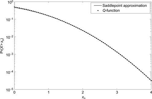
Figure 4.6 The Q-function and its saddle point approximation.
4.11 Engineering Application—Scalar Quantization
In many applications, it is convenient to convert a signal which is analog in nature to a digital one. This is typically done in three steps. First, the signal is sampled, which converts the signal from continuous time to discrete time. Then samples of the signal are quantized. This second action converts the signal from one with a continuous amplitude to one whose amplitude can only take on discrete values. Once the signal is converted to discrete time/discrete amplitude, the signal can then easily be represented by a sequence of bits. In this third step, each discrete amplitude level is represented by a binary codeword. While the first step (sampling) and the third step (encoding) are invertible, the second step (quantization) is not. That is, we can perfectly recover the analog signal from its discrete time samples (provided the samples are taken at a rate above the Nyquist rate), and the discrete amplitude levels can easily be recovered from the codewords which represent them (provided a lossless source code is used). However, the act of quantization causes distortion of the signal which cannot be undone. Given the discrete amplitude of a sample, it is not possible to determine the exact value of the original (continuous amplitude) sample. For this reason, careful attention is paid to the quantization process in order to minimize the amount of distortion.
In order to determine efficient ways to quantize signals, we must first quantify this concept of signal distortion. Suppose a signal is sampled and we focus attention on one of those samples. Let the random variable X represent the value of that sample, which in general will draw from a continuous sample space. Now suppose that sample is quantized (using some quantization function q(x)) to form a new (discrete) random variable Y = q(X). The difference between the original sample value and its quantized value, X − q(X), is the error caused by the quantizer, or the quantizer noise. It is common to measure signal distortion as the mean-squared quantizer error,
![]() (4.77)
(4.77)
We will see in Chapter 10 that the mean-squared value of a signal has the physical interpretation of the signal’s power. Thus, the quantity d can be interpreted as the quantization noise power. Often the fidelity of a quantized signal is measured in terms of the ratio of the original signal power, E[X2], to the quantization noise power. This is referred to as the signal-to-quantization-noise power ratio (SQNR)
![]() (4.78)
(4.78)
The goal of the quantizer design is to choose a quantization function which minimizes the distortion, d. Normally, the quantizer maps the sample space of X into one of M = 2n levels. Then each quantization level can be represented by a unique n-bit codeword. We refer to this as an n-bit quantizer. As indicated in Equation (4.77), the expected value is with respect to the PDF of X. Hence, the function q(x) that minimizes the distortion will depend on the distribution of X.
To start with consider a random variable X which is uniformly distributed over the interval (−a/2, a/2). Since the sample X is equally likely to fall anywhere in the region, it would make sense for the quantizer to divide that region into M equally spaced subintervals of width Δ = a/M. For each subinterval, the quantization level (i.e., the value of q(x) for that subinterval) should be chosen as the midpoint of the subinterval. This is referred to as a uniform quantizer. A 3-bit uniform quantizer is illustrated in Figure 4.7. For example, if X ∈ (0, a/8), then q(X) = a/16. To measure the distortion for this signal together with the uniform quantizer, condition on the event that the signal falls within one of the quantization intervals, and then use the theorem of total probability:

Figure 4.7 A 3-bit uniform quantizer on the interval (– a/2, a/2).
 (4.79)
where Xk refers to the kth quantization interval. Consider, for example, X5 = (0, a/8), so that
![]() (4.80)
(4.80)
To calculate this conditional expected value requires the conditional PDF of X. From Equation (3.41) this is
![]() (4.81)
(4.81)
Not surprisingly, conditioned on X ∈ (0, a/8), X is uniformly distributed over (0, a/8). The conditional expected value is then
 (4.82)
Due to the symmetry of the uniform distribution, this conditional distortion is the same regardless of what quantization interval the signal falls in. Hence, Equation (4.82) is also the unconditional distortion. Note that the power of the original signal is
 (4.83)
The resulting SQNR is then
![]() (4.84)
(4.84)
The preceding result for the three-bit uniform quantizer can be generalized to any uniform quantizer. In general, for an n-bit uniform quantizer, there will be M = 2n quantization intervals of width Δ = a/M. Consider the quantization interval (0, Δ) and suppose the quantization level for that interval is chosen to be the midpoint, Δ 2. Then the distortion for that interval (and hence the distortion for the quantizer) is
 (4.85)
The SQNR for an n-bit uniform quantizer with a uniformly distributed input is
![]() (4.86)
(4.86)
This is the so-called 6 dB rule whereby the SQNR is increased by approximately 6 dB for each extra bit added to the quantizer. For example, in wireline digital telephony, 8-bit quantization is used which would result in an SQNR of approximately 48 dB.
The previous results assumed that the input to the quantizer followed a uniform probability distribution. This is rarely the case. Speech signals, for example, are commonly modeled using a Laplace (two-sided exponential) distribution. For such signals, small sample values are much more frequent than larger values. In such a situation, it would make sense to use finer resolution (i.e., narrower quantization intervals) for the most frequent smaller amplitudes in order to keep the distortion minimized in those regions, at the cost of more distortion in the less frequent larger amplitude regions.
Given that an n-bit quantizer is to be used, the design of an optimum quantizer involves two separate problems. First, the ranges for each quantization interval must be specified; then the quantization level for each interval must be chosen. The following theorem specifies how each of these two tasks should be accomplished.
Theorem 4.9: A random variable X with PDF fx(x) is to be quantized with an M-level quantizer that produces a discrete random variable Y according to
![]() (4.87)
(4.87)
where it is assumed that the lower limit of the first quantization interval is x0 = −∞ and the upper limit of the last quantization interval is xM = ∞. The (mean-squared) distortion is minimized by choosing the quantization intervals (i.e., the xi) and the quantization levels (i.e., the yi) according to
(i) ![]() (4.88)
(4.88)
(ii) ![]() (4.89)
(4.89)
These two criteria provide a system of 2M − 1 equations with which to solve for the 2M − 1 quantities (x1, x2, …, xM−1, y1, y2, …, yM) which specify the optimum M-level quantizer.
Proof: The distortion is given by
 (4.90)
To minimize d with respect to yj,
 (4.91)
Solving for yj in this equation establishes the conditional mean criterion. Similarly differentiating with respect to xj gives
![]() (4.92)
(4.92)
Solving for xj produces the midpoint criterion.
Example 4.30
Using the criteria set forth in Theorem 4.9, an ideal nonuniform 2-bit quantizer will be designed for a signal whose samples have a Laplace distribution, fx(x) = (1/2)exp(−|x|). A 2-bit quantizer will have four quantization levels, {y1, y2, y3, y4}, and four corresponding quantization intervals which can be specified by three boundary points, {x1, x2, x3}. The generic form of the 2-bit quantizer is illustrated in Figure 4.8. Due to the symmetry of the Laplace distribution, it seems reasonable to expect that the quantizer should have a negative symmetry about the y-axis. That is, x1 = −x3, x2 = 0, y1 = −y4, and y2 = −y3. Hence, it is sufficient to determine just three unknowns, such as {x3, y3, y4}. The rest can be inferred from the symmetry. Application of the conditional mean criterion and the midpoint criterion leads to the following set of three equations:


Figure 4.8 A 2-bit quantizer.
Plugging the expressions for y3 and y4 into the last equation results in a single equation to solve for the variable x3. Unfortunately, the equation is transcendental and must be solved numerically. Doing so results in the solution {x3, y3, y4} = {1.594, 0.594, 2.594}. The (mean-squared) distortion of this 2-bit quantizer is given by
![]()
Note that the power in the original (unquantized) signal is E[X2] = 2 so that the SQNR of this quantizer is
![]()
Example 4.31
In this example, we generalize the results of the last example for an arbitrary number of quantization levels. When the number of quantization levels get large, the number of equations to solve becomes too difficult to do by hand, so we use MATLAB to help us with this task. Again, we assume that the random variable X follows a Laplace distribution given by fx(x) = (1/2)exp(−|x|). Because of the symmetry of this distribution, we again take advantage of the fact that the optimum quantizer will be symmetric. We design a quantizer with M levels for positive X (and hence M levels for negative X as well, for a total of 2M levels). The M quantization levels are at y1, y2,…, yM and the quantization bin edges are at x0= 0, x1, x2, …, xN−1, xN = ∞. We compute the optimum quantizer in an iterative fashion. We start by arbitrarily setting the quantization bins in a uniform fashion. We choose to start with xi = 2i/ M. We then iterate between computing new quantization levels according to Equation (4.88) and new quantization bin edges according to Equation (4.89). After going back and forth between these two equations several times, the results converge toward a final optimum quantizer. For the Laplace distribution, the conditional mean criterion results in
![]()
At each iteration stage (after computing new quantization levels), we also compute the the SQNR. By observing the SQNR at each stage, we can verify that this iterative process is in fact improving the quantizer design at each iteration. For this example, the SQNR is computed according to (see Exercise 4.82).

The MATLAB code we used to implement this process is included below. Figure 4.9 shows the results of running this code for the case of M = 8 (16 level, 4-bit quantizer).

Figure 4.9 SQNR measurements for the iterative quantizer design in Example 4.31. (For color version of this figure, the reader is refered to the web version of this chapter).

4.12 Engineering Application—Entropy and Source Coding
The concept of information is something we hear about frequently. After all, we supposedly live in the “information age” with the internet is often referred to as the “information superhighway.” But, what is information? In this section, we give a quantitative definition of information and show how this concept is used in the world of digital communications. To motivate the forthcoming definition, imagine a situation where we had a genie who could tell us about certain future events. Suppose that this genie told us that on July 15th of next year, the high temperature in the state of Texas would be above 90° F. Anyone familiar with the weather trends in Texas would know that our genie has actually given us very little information. Since we know that the temperature in July in Texas is above 90°F with probability approaching one, the statement made by the genie does not tell us anything new. Next, suppose that the genie tells us that on July 15th of next year, the high temperature in the state of Texas would be below 80° F. Since this event is improbable, in this case the genie would be giving us a great deal of information.
To define a numerical quantity which we will call information, we note from the previous discussion that
• Information should be a function of various events. Observing (or being told) that some event A occurs (or will occur) provides a certain amount of information, I(A).
• The amount of information associated with an event should be inversely related to the probability of the event. Observing highly probable events provides very little information, while observing very unlikely events gives a large amount of information.
At this point, there are many definitions which could satisfy the two previous bullet items. We include one more observation that will limit the possibilities:
• If it is observed that two events, A and B, have occurred and if those two events are independent, then we expect that the information I(A ∩B) = I(A) + I(B).
Since we observed that information should be a function of the probability of an event, the last bullet item requires us to define information as a function of probability that satisfies
![]() (4.93)
(4.93)
Since a logarithmic function satisfies this property, we obtain the following definition.
Definition 4.11: If some event A occurs with probability pA, then observing the event A provides an amount of information given by
![]() (4.94)
(4.94)
The units associated with this measure of information depend on the base of the logarithm used. If base 2 logs are used, then the unit of information is a “bit”; if natural logs are used, the unit of information is the “nat.”
Note that with this definition, an event which is sure to happen (pA = 1) provides I(A) = 0 bits of information. This makes sense since if we know the event must happen, observing that it does happen provides us with no information.
Next, suppose we conduct some experiment which has a finite number of outcomes.
The random variable X will be used to map those outcomes into the set of integers,
0, 1, 2, …, n − 1. How much information do we obtain when we observe the outcome of the experiment? Since information is a function of the probability of each outcome, the amount of information is random and depends on which outcome occurs. We can, however, talk about the average information associated with the observation of the experiment.
Definition 4.12: Suppose a discrete random variable X takes on the values 0, 1, 2, …, n − 1 with probabilities p0, p1, …, pn−1. The average information or (Shannon) entropy associated with observing a realization of X is
 (4.95)
Entropy provides a numerical measure of how much randomness or uncertainty there is in a random variable. In the context of a digital communication system, the random variable might represent the output of a data source. For example, suppose a binary source outputs the letters X = 0 and X = 1 with probabilities p and 1 − p, respectively. The entropy associated with each letter the source outputs is
![]() (4.96)
(4.96)
The function H(p) is known as the binary entropy function and is plotted in Figure 4.10. Note that this function has a maximum value of 1 bit when p = 1/2. Consequently, to maximize the information content of a binary source, the source symbols should be equally likely.

Figure 4.10 The binary entropy function.
Next, suppose a digital source described by a discrete random variable X periodically outputs symbols. Then the information rate of the source is given by H(X) bits/source symbol. Furthermore, suppose we wish to represent the source symbols with binary codewords such that the resulting binary representation of the source outputs uses r bits/symbol. A fundamental result of source coding, which we will not attempt to prove here, is that if we desire the source code to be lossless (that is, we can always recover the original source symbols from their binary representation), then the source code rate must satisfy r ≥ H(X). In other words, the entropy of a source provides a lower bound on the average number of bits that are needed to represent each source output.
Example 4.32
Consider a source that outputs symbols from a four-letter alphabet. That is, suppose X ∈ {a, b, c, d}. Let pa = 1/2, pb = 1/4, and pc = pd = 1/8 be the probability of each of the four source symbols. Given this source distribution, the source has an entropy of
![]()
Table 4.2 shows several different possible binary representations of this source. This first code is the simplest and most obvious representation. Since there are four letters, we can always assign a unique 2-bit codeword to represent each source letter. This results in a code rate of r1 = 2 bits/symbol which is indeed greater than the entropy of the source. The second code uses variable length codewords. The average codeword length is
![]()
Table 4.2. Three possible codes for a four-letter source

Therefore, this code produces the most efficient representation of any lossless source coded since the code rate is equal to the source entropy. Note that Code 3 from Table 4.2 produces a code rate of
![]()
which is lower than the entropy, but this code is not lossless. This can easily be seen by noting that the source sequences “d” and “a, b” both lead to the same encoded sequence “01.”
Exercises
Section 4.1: Expected Values of a Random Variable
4.1 Find the mean of the random variables described by each of the following probability density functions:
4.2 Find the mean of the random variables described by each of the following probability mass functions:
4.3 Find the mean of the random variables described by each of the following cumulative distribution functions:


4.4 In each of the following cases, find the value of the parameter a which causes the indicated random variable to have a mean value of 10.


4.5 Suppose a random variable X has a PDF which is nonzero only on the interval [0, ∞). That is, the random variable cannot take on negative values. Prove that
![]()
Section 4.2: Expected Values of Functions of a Random Variable
4.6 Two players compete against each other in a game of chance where Player A wins with probability 1/3 and Player B wins with probability 2/3. Every time Player A loses he must pay Player B $1, while every time Player B loses he must pay Player A $3. Each time the two play the game, the results are independent of any other game. If the two players repeat the game 10 times, what is the expected value of Player A’s winnings?
4.7 The current flowing through a 75 Ω resistor is modelled as a Gaussian random variable with parameters, m = 0A and σ = 15 mA. Find the average value of the power consumed in the resistor.
4.8 The received voltage in a 75 Ω antenna of a wireless communication system is modeled as a Rayleigh random variable, ![]() . What does the value of the parameter σ need to be for the received power to be 10 μW?
. What does the value of the parameter σ need to be for the received power to be 10 μW?
4.9 Suppose X is a Gaussian random variable with a mean of μ and a variance of σ2 (i.e., X∼N(μ, σ2)). Find an expression for E[|X|].
4.10 Prove Jensen’s inequality, which states that for any convex function g(x) and any random variable X,
![]()
Section 4.3: Moments
4.11 Find an expression for the m th moment of an Erlang random variable whose PDF is given by ![]() for some positive integer n and positive constant b.
for some positive integer n and positive constant b.
4.12 Find an expression for the even moments of a Rayleigh random variable. That is, find E[Y2m] for any positive integer m if the random variable, Y, has a PDF given by ![]() .
.
4.13 Find the first three moments of a geometric random variable whose PMF is PN(n) = (1 − p)pn, n = 0, 1, 2,….
4.14 Find the first three moments of a Poisson random variable whose PMF is ![]() .
.
4.15 For the Rayleigh random variable described in Exercise 4.12, find a relationship between the nth moment, E[Yn], and the nth moment of a standard normal random variable.
4.16 Suppose X is a random variable whose n th moment is gn, n = 1, 2, 3…. In terms of the gn, find an expression for the m th moment of the random variable Y = aX+ b for constants a and b.
4.17 Suppose X is a random variable whose nth moment is gn, n = 1, 2, 3…. In terms of the gn, find an expression for E[eX].
Section 4.4: Central Moments
4.18 Calculate the mean value, second moment, and variance of each of the following random variables:

4.19 For a Gaussian random variable, derive expressions for the coefficient of skewness and the coefficient of kurtosis in terms of the mean and variance, μ and σ2.
4.20 Prove that all odd central moments of a Gaussian random variable are equal to zero. Furthermore, develop an expression for all even central moments of a Gaussian random variable.
4.21 Show that the variance of a Cauchy random variable is undefined (infinite).
4.22 Let cn be the n th central moment of a random variable and μn be its n th moment. Find a relationship between cn and μk, k = 0, 1, 2, …, n.
4.23 Let X be a random variable with E[X] = 1 and var(X) = 4. Find the following:
4.24 A random variable X has a uniform distribution over the interval (−a/2, a/2) for some positive constant a.
(a) Find the coefficient of skewness for X;
(b) Find the coefficient of kurtosis for X;
(c) Compare the results of (a) and (b) with the same quantities for a standard normal random variable.
4.25 Suppose Θ is a random variable uniformly distributed over the interval [0, 2π).
4.26 A random variable has a CDF given by

4.27 Find the variance and coefficient of skewness for a geometric random variable whose PMF is PN(n) = (1 − p)pn, n = 0, 1, 2,…. Hint: You may want to use the results of Exercise 4.13.
4.28 Find the variance and coefficient of skewness for a Poisson random variable whose PMF is ![]() . Hint: You may want to use the results of Exercise 4.14.
. Hint: You may want to use the results of Exercise 4.14.
Section 4.5: Conditional Expected Values
4.29 Show that the concept of total probability can be extended to expected values. That is, if {Ai}, i = 1, 2, 3, …, n is a set of mutually exclusive and exhaustive events, then

4.30 An exponential random variable has a PDF given by fX(x) = exp(−x)u(x).
(a) Find the mean and variance of X.
(b) Find the conditional mean and the conditional variance given that X > 1.
4.31 A uniform random variable has a PDF given by fX(x) = u(x) − u (x−1).
(a) Find the mean and variance of X.
(b) Find the conditional mean and the conditional variance given that ![]() .
.
4.32 Consider a Gaussian random variable, X, with mean μ and variance σ2.
4.33 A professor is studying the performance of various student groups in his class. Let the random variable X represent a students final score in the class and define the following conditioning events:
(a) Suppose the average score among males is E[X|M] = 73.2 and the average score among females is E[X|F] = 75.8. If the overall class average score is E[X] = 74.6, what percentage of the class is female?
(b) Suppose the conditional average scores by class are E[X|F] = 65.8, E[X|So] = 71.2, E[X|J] = 75.4, E[X|Se] = 79.1. If the overall class average score is E[X] = 72.4, what can we say about the percentage of freshmen, sophomore, juniors and seniors in the class?
(c) Given the class statistics in part (b). If it is known that there are 10 freshmen, 12 sophomores, and 9 juniors in the class, how many seniors are in the class?
Section 4.6: Transformations of Random Variables
4.34 Suppose X is uniformly distributed over (−a, a), where a is some positive constant. Find the PDF of Y = X2.
4.35 Suppose X is a random variable with an exponential PDF of the form fX(x) = 2e−2x u(x). A new random variable is created according to the transformation Y = 1 − X.
4.36 Let X be a standard normal random variable (i.e., X ∼ N(0, 1)). Find the PDF of Y = |X|.
4.37 Repeat Exercise 4.36 if the transformation is

4.38 Suppose a random variable, X, has a Gaussian PDF with zero mean and variance σX2. The random variable is transformed by the device whose input–output relationship is shown in the accompanying figure. Find and sketch the PDF of the transformed random variable, Y.
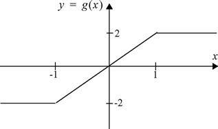
4.39 Let X be a Gaussian random variable with zero mean and arbitrary variance, σ2. Given the transformation Y = X3, find fY(y).
4.40 A real number between 0 and 100 is randomly selected according to a uniform distribution and rounded off to the nearest integer. For example, 36.5001 is rounded off to 37; ![]() is rounded off to 2; and 69.49 is rounded off to 69. Define a random variable to be X = (number selected) – (nearest integer).
is rounded off to 2; and 69.49 is rounded off to 69. Define a random variable to be X = (number selected) – (nearest integer).
4.41 A Gaussian random variable with zero mean and variance σX2 is applied to a device that has only two possible outputs, 0 or 1. The output 0 occurs when the input is negative, and the output 1 occurs when the input is nonnegative.
4.42 Let X be a Cauchy random variable whose PDF is given by
![]()
4.43 Let X be a Chi-square random variable with a PDF given by
![]()
where c = n/2 for any positive integer n. Find the PDF of ![]() .
.
4.44 Suppose a random variable has some PDF given by fX(x). Find a function g(x) such that Y = g(X) is a uniform random variable over the interval (0, 1). Next, suppose that X is a uniform random variable. Find a function g(x) such that Y = g(X) has some specified PDF, fY(y).
4.45 Suppose X is uniformly distributed over (0, 1). Using the results of Exercise 4.44, find transformations Y = g(X) to produce random variables with the following distributions:
4.46 Suppose X is a binomial random variable with parameters n and p. That is, the PMF of X is given by
![]()
Find the PMF of a new random variable generated through the transformation, Y = n−X.
4.47 Suppose X is a Gaussian random variable with mean μX and variance σX2. Suppose we form a new random variable according to Y = aX + b for constants a and b.
(a) Prove that Y is also Gaussian for any a ≠ 0.
(b) What values for the constants a and b will lead to the new random variable Y having zero mean and unit variance?
(c) What values for the constants a and b will lead to the new random variable Y having a mean of μY and a variance of σY2?
4.48 The amplitude, A, of a received signal in a wireless communication system is often modelled as a Rayleigh random variable whose PDF is of the form, ![]() . The (normalized) power of the same signal is given by P = A2. Find the PDF of P.
. The (normalized) power of the same signal is given by P = A2. Find the PDF of P.
4.49 Suppose X is an exponential random variable with PDF, fX(x) = exp (−x)u(x). Find a transformation, Y = g(X) so that the new random variable Y has a Cauchy PDF given by ![]() . Hint: Use the results of Exercise 4.44.
. Hint: Use the results of Exercise 4.44.
Section 4.7: Characteristic Functions
4.50 A random variable X has a characteristic function, ϕX(ω). Write the characteristic function of Y = aX+ b in terms of ϕX(ω) and the constants a and b.
4.51 Prove that the characteristic function of any random variable must satisfy the following properties.
4.52 Suppose X is an integer-valued random variable. Show that in this case, ϕX(2 πn) = 1 for any integer, n. Likewise, prove the reverse is also true. That is, show that if ϕX(27πn) = 1 for any integer, n, the random variable X must be integer-valued.
4.53 For a Laplace random variable whose PDF is given by ![]() , find the following:
, find the following:
4.54 An Erlang Random variable has a PDF of the form ![]() .
.
4.55 A Cauchy random variable has a PDF ![]() .
.
(a) Find the characteristic function, ϕX(ω).
(b) Show that the derivatives ![]() do not exist at ω = 0. What does this mean?
do not exist at ω = 0. What does this mean?
4.56 A Poisson random variable has a PMF of the form ![]() , k = 0, 1, 2,….
, k = 0, 1, 2,….
(a) Find the characteristic function, ϕX(ω).
(b) Find the first three nonzero terms in the Taylor series expansion of ln[ϕX(ω)].
(c) Use the results of part (b) to find the mean, variance, and skewness of the Poisson random variable.
4.57 A certain random variable has a characteristic function given by
![]()
Find the PDF of this random variable.
4.58 Which of the following functions could be the characteristic function of a random variable? See Appendix E, Section 5 for definitions of these functions.
Section 4.8: Probability-Generating Functions
4.59 Derive a formula expressing the variance of a random variable in terms of its factorial moments.
4.60 Derive a relationship between the k th factorial moment for a nonnegative, integer-valued random variable and the coefficients of the Taylor series expansion of its probability-generating function, HX(z), about the point z = 1.
4.61 For a Poisson random variable whose PMF is given by, ![]() k = 0, 1, 2, …, find the following:
k = 0, 1, 2, …, find the following:
(a) the probability-generating function, HX(z),
(b) the Taylor series expansion of HX(z) about the point z = 1,
4.62 A certain random variable has a probability-generating function given by
![]()
Find the PMF for this random variable.
4.63 Show that for any probability-generating function, H(z), H(1) = 1.
4.64 Suppose HX(z) is the probability-generating function of some random variable X with PMF PX(k). In terms of PX(k), find the PMF of the random variable Y if its probability-generating function is given as in each of the following cases.
Section 4.9: Moment-Generating Functions
4.65 Derive an expression for the moment-generating function of a Rayleigh random variable whose PDF is
![]()
4.66 Suppose X is a Rician random variable with a PDF given by
![]()
Derive an expression for E[euX2]. Note that this is not quite the moment-generating function, but it can be used in a similar way.
4.67 A Gaussian mixture is a random variable whose PDF is a linear combination of two Gaussian PDFs,

(a) Find the moment-generating function, MX(u), of the Gaussian mixture.
(b) Use the moment-generating function to find the mean of the Gaussian mixture.
4.68 A random variable has a moment-generating function given by
![]()
(a) Find the PDF of the random variable.
(b) Use the moment-generating function to find an expression for the k th moment of the random variable.
4.69 Consider a moment-generating function of the general form
![]()
for constants a, b, and c. Find constraints that the constants a, b, and c must satisfy so that MX(u) is the MGF of a valid random variable.
4.70 Prove the following properties of moment-generating functions.
4.71 Find the mean of the random variable whose moment-generating function is
![]()
Section 4.10: Evaluating Tail Probabilities
4.72 Prove that for a random variable X with mean μX,
![]()
where n is any positive integer.
4.73 Suppose we are interested in finding the left tail probability for a random variable, X. That is, we want to find Pr(X≤xo). Rederive an expression for the Chernoff bound for the left tail probability.
4.74 Suppose X is a Poisson random variable with PMF, ![]() , k = 0, 1, 2,…. Find the Chernoff bound for the tail probability, Pr(X≥no).
, k = 0, 1, 2,…. Find the Chernoff bound for the tail probability, Pr(X≥no).
4.75 Suppose X is a Gamma random variable with PDF, ![]() . Find the Chernoff bound for the tail probability, Pr(X>xo).
. Find the Chernoff bound for the tail probability, Pr(X>xo).
4.76 Let X be an Erlang random variable with PDF, ![]() . Derive a saddle point approximation for the left tail probability, Pr(X ≤ xo). Compare your result with the exact value for 0 ≤ xo ≤ E[X].
. Derive a saddle point approximation for the left tail probability, Pr(X ≤ xo). Compare your result with the exact value for 0 ≤ xo ≤ E[X].
4.77 In Exercise 4.66, an expression was derived for E[euX2] for a Rician random variable. Use this function to obtain a saddle point approximation for the tail probability of a Rician random variable, Pr(X ≥ xo).
Hint: For one-sided random variables, Pr(X ≥ xo) = Pr(X2 ≥ x2o).
4.78 The average number of cars per hour arriving at a toll booth is 57 while the standard deviation is 15.
(a) Use Markov’s inequality to find an upper bound on the probability of having more than 200 cars arrive in an hour.
(b) Use Chebyshev’s inequality to find an upper bound on the probability of having more than 200 cars arrive in an hour.
4.79 In a certain communication system, bits are encoded into blocks of length 128 bits. Error correction techniques are used such that the block will be decoded correctly as long as no more than 7 of the 128 bits are received in error. We observe that 2% of our blocks are decoded incorrectly. From Markov’s inequality, what can we say about the average number of bit errors that occur in each 128 bit block?
4.80 A nonnegative random variable X has moments which are known to be E[X] = 1, E[X2] = 2, E[X3] = 5, E[X4] = 9, E[X5] = 14, E[X6] = 33.
(a) Show that for any nonnegative random variable, ![]() .
.
(b) Using the result of part (a) and the values of the moments given, find the tightest bound on Pr(X≥ 2).
(c) Using the result of part (a) and the values of the moments given, find the tightest bound on Pr(X ≥ 3).
4.81 Since the Q-function represents the tail probability of a Gaussian random variable, we can use the various bounds on tail probabilities to produce bounds on the Q-function.
(a) Use Markov’s inequality to produce an upper bound on the Q-function. Hint: a Gaussian random variable has a two-sided PDF, and Markov’s inequality requires the random variable to be one-sided. You will need to work with absolute values to resolve this issue.
(b) Use Chebyshev’s inequality to produce an upper bound on the Q-function.
(c) Plot your results from parts (a) and (b) along with the bound obtained from the Chernoff bound from Example 4.28. In order to determine how tight (or loose) these various bounds are, also include on your plot the exact value of the Q-function.
Section 4.11: Scalar Quantization
4.82 Consider a quantizer that is designed to minimize the mean square quantization error. That is, the quantization levels, yi, are chosen according to the conditional mean criterion and the bin edges, xi, are chosen according to the midpoint criterion. Show that the distortion is given by
and therefore the SQNR can be written as

4.83 Following the lead of Example 4.30, design an optimum 2-bit quantizer for a signal whose samples follow a triangular PDF,

Section 4.12: Entropy and Source Coding
4.84 Suppose a source sends symbols from a three letter alphabet with X ∈ {a, b, c} and pa = 1/2, pb = 1/4, pc = 1/4 are the source symbol probabilities.
(a) Determine the entropy of this source.
(b) Give a source code that has an average codeword length that matches the entropy.
4.85 Suppose a random variable, X, has N = 2n equally likely outcomes. What is the entropy of X in bits?
4.86 Suppose a fair coin is flipped n times and the random variable Y counts the number of times heads occurs. What is the entropy of Y in bits? Compare your answer to that of Exercise 4.85 and explain any difference.
4.87 Consider an N-letter source with probabilities, pi, i = 1, 2, 3, …, N. The entropy of the source is given by  . Prove that the discrete distribution that maximizes the entropy is a uniform distribution. Hint: You need to perform a constrained optimization since the source probabilities must form a valid probability mass function, and thus p1 +p2 + … + pN = 1.
4.88 Consider a geometric random variable, Z, whose PMF is PZ(k) = (1−p)pk, k = 0, 1, 2,…. Find the entropy of this random variable as a function of p.
Miscellaneous Exercises
4.89 Imagine that you are trapped in a circular room with three doors symmetrically placed around the perimeter. You are told by a mysterious voice that one door leads to the outside after a 2-h trip through a maze. However, the other two doors lead to mazes that terminate back in the room after a 2-h trip at which time you are unable to tell through which door you exited or entered. What is the average time for escape to the outside? Can you guess the answer ahead of time? If not, can you provide a physical explanation for the answer you calculate?
4.90 A communication system sends data in the form of packets of fixed length. Noise in the communication channel may cause a packet to be received incorrectly. If this happens, then the packet is retransmitted. Let the probability that a packet is received incorrectly be q. Determine the average number of transmissions that are necessary before a packet is received correctly.
4.91 In Exercise 4.90 let the transmission time be Tt seconds for a packet. If the packet was received incorrectly, then a message is sent back to the transmitter that states that the message was received incorrectly. Let the time for sending such a message be Ti. Assume that if the packet is received correctly that we do not send an acknowledgement. What is the average time for a successful transmission?
4.92 Use the characteristic function (or the moment-generating function or the probability-generating function) to show that a Poisson PMF is the limit of a binomial PMF with n approaching infinity and p approaching zero in such a way that np = μ = constant.
MATLAB Exercises
4.93 Let X be a random variable that is uniformly distributed over the interval (0, 100). Form a new random variable Y by rounding X to the nearest integer. In MATLAB code, this could be represented by Y=round(X). Finally, form the random roundoff error according to Z = X − Y.
(a) Using analytical methods, find the PDF of Z as well as the mean-squared value, E[Z2].
(b) Using MATLAB, create a histogram for the probability densities for the random variable Z. Compare with the PDF found analytically in part (a).
4.94 Suppose you have a random variable X with PDF, fX(x) = 2x(u(x) − u(x − 1)) and that this random variable is transformed as Y = 2 − X. Calculate fY(y). Repeat this problem using MATLAB. Compare the estimate of the PDF from MATLAB with the analytically determined PDF. Note that for this problem there is no function in MATLAB that provides a sequence of data samples that has the PDF specified in this problem for X. Thus you must find an appropriate way to transform a uniform random variable to produce the desired X. The results of Exercise 4.44 will be helpful here.
4.95 Use MATLAB to generate a large number of samples from a Gaussian distribution with mean μ = 20 and variance σ = 4. Hint: the MATLAB command sigma*randn(1, N)+mu will create N such numbers with mean mu and standard deviation sigma. Let x1, x2, …, xN represent the samples you generated. Compute each of the following “mean” values:


(d) Quadratic mean (root mean square), 
Which of these “estimates” give a decent estimate of the true mean?
4.96 Write a MATLAB program to simulate the problem described in Exercise 4.89. Estimate the average time until escape. Do your MATLAB results agree with your analytically determined results in Exercise 4.89?
4.97 Copy a segment of text into MATLAB as a string (you choose the source of the text). Then write a MATLAB program to count the relative frequency of each character (ignore all characters that do not correspond to one of the 26 letters and do not make a distinction between upper and lower case). Using the results of your program, calculate the entropy of a source that outputs the 26 English characters with the probabilities you calculated.
4.98 Suppose a random variable has a PDF given by

Following the procedure laid out in Example 4.31, write a MATLAB program to design an optimum 4-bit (16 level) quantizer for this random variable. Compute the SQNR in decibels of the quantizer you designed. How does this SQNR compare with that obtained in Example 4.31. Can you explain any differences?
1 Note that this definition assumes that the discrete random variable, X, is defined on nonnegative integer values, k. One could also define a probability-generating function based on a bilateral z-transform which would allow for random variables which can take on negative integer values as well. However, since this is less common, we do not consider it further here.
2 One may also define a moment-generating function for random variables which are not necessarily nonnegative. In that case, a two-sided Laplace transform would be appropriate. This would be identical to the characteristic function with the association u = jω.
3 The remainder of this section assumes the student is familiar with the concepts of contour integration and residue calculus. For those students not familiar with these topics, the remainder of this section can be skipped without any loss in continuity.