
CHAPTER 12
Simulation Techniques
With the increasing computational power of very inexpensive computers, simulation of various systems is becoming very common. Even when a problem is analytically tractable, sometimes it is easier to write a quick program to simulate the desired results. However, there is a certain art to building good simulations, and many times avoidable mistakes have led to incorrect simulation results. This chapter aims at helping the reader to build a basic knowledge of some common techniques used for simulation purposes. Most of the results presented in this chapter are just applications of material covered in previous chapters, so there is nothing fundamentally new here. Nevertheless, armed with some of the basic simulation principles presented in this chapter, the reader should be able to develop simulation tools with confidence.
12.1 Computer Generation of Random Variables
In this section, we study techniques used to generate random numbers. However, we must start with a disclaimer. Most of the techniques used in practice to generate so-called random numbers will actually generate a completely deterministic sequence of numbers. So, what is actually random about these random number generators? Strictly speaking, nothing! Rather, when we speak of computer-generated random numbers, we are usually creating a sequence of numbers that have certain statistical properties that make them behave like random numbers, but in fact they are not really random at all. Such sequences of numbers are more appropriately referred to as pseudorandom numbers.
12.1.1 Binary Pseudorandom Number Generators
To start with, suppose we would like to simulate a sequence of independent identically distributed (IID) Bernoulli random variables, X1, X2, X3, …. One way to do this would be to grab a coin and start flipping it and observe the sequence of heads and tails, which could then be mapped to a sequence of 1s and 0 s. One drawback to this approach is that it is very time consuming. If our application demanded a sequence of length 1 million, not many of us would have the patience to flip the coin that many times. Therefore, we seek to assign this task to a computer. So, to simulate an IID sequence of random variables, essentially we would like to create a computer program that will output a binary sequence with the desired statistical properties. For example, in addition to having the various bits in the sequence be statistically independent, we might also want 0 s and 1s to be equally likely.
Consider the binary sequence generated by the linear feedback shift register (LFSR) structure illustrated in Figure 12.1. In that figure, the square boxes represent binary storage elements (i.e., flip-flops) while the adder is modulo-2 (i.e., an exclusive OR gate). Suppose the shift register is initially loaded with the sequence 1, 1, 1, 1. It is not difficult to show that the shift register will output the sequence
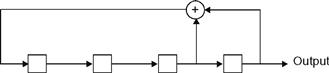
Figure 12.1 A four-stage, binary linear feedback shift register.
![]() (12.1)
(12.1)
If the shift register were clocked longer, it would become apparent that the output sequence would be periodic with a period of 15 bits. While periodicity is not a desirable property for a pseudorandom number generator, if we are interested in generating short sequences (of length less than 15 bits), then the periodicity of this sequence generator would not come into play. If we are interested in generating longer sequences, we could construct a shift register with more stages so that the period of the resulting sequence would be sufficiently long so that its periodicity would not be of concern.
The sequence generated by our LFSR does possess several desirable properties. First, the number of 1s and 0 s is almost equal (eight 1s and seven 0 s is as close as we can get to equally likely with a sequence of length 15). Second, the autocorrelation function of this sequence is nearly equal to that of a truly random binary IID sequence (again, it is as close as we can possibly get with a sequence of period 15; see Exercise 12.1). Practically speaking, the sequence output by this completely deterministic device does a pretty good job of mimicking the behavior of an IID binary sequence. It also has the advantage of being repeatable. That is, if we load the shift register with the same initial contents, we can always reproduce the exact same sequence.
It should be noted that not all LFSRs will serve as good pseudorandom number generators. Consider for example the four-stage LFSR in Figure 12.2. This shift register is only a slightly modified version of the one in Figure 12.1, yet when loaded with the sequence 1, 1, 1, 1, this shift register outputs a repeating sequence of all 1s (i.e., the period of the output sequence is 1). The only difference between the two shift registers is in the placement of the feedback tap connections. Clearly, the placement of these tap connections is crucial in creating a good pseudorandom sequence generator.
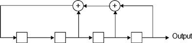
Figure 12.2 Another four-stage, binary linear feedback shift register.
A general N-stage LFSR is shown in Figure 12.3. The feedback tap gains, gi , i = 0, 1, 2, …, N, are each either 0 or 1. A 1 represents the presence of a tap connection, while a 0 represents the absence of a tap connection. It is also understood that g0 = gN = 1. That is, there must always be connections at the first and last position. A specific LFSR can then be described by the sequence of tap connections. For example, the four stage LFSR in Figure 12.1 can be described by the sequence of tap connections [g0, g1, g2, g3, g4] = [1, 0, 1, 1, 1] It is also common to further simplify this shorthand description of the LFSR by converting the binary sequence of tap connections to an octal number. For example, the sequence [1, 0, 0, 1, 1] becomes the octal number 23. Likewise, the LFSR in Figure 12.2 is described by [g0, g1, g2, g3, g4] = [1, 0, 1, 1, 1] → 27.

Figure 12.3 A general N-stage, binary linear feedback shift register.
An N-stage LFSR must necessarily generate a periodic sequence of numbers. At any point in time, the N-bit contents of the shift register can take on only one of 2N possibilities. Given any starting state, the LFSR could at best cycle through all possible states, but sooner or later must return to its initial state (or some other state it has already been in). At that point, the output will then begin to repeat itself. Also, note that if the LFSR ever gets into the all zero state, it will remain in that state and output a sequence of all 0 s from that point on. Therefore, to get the maximum period out of a LFSR, we would like the shift register to cycle through all possible non-zero states exactly once before returning to its initial state. This will produce a periodic output sequence with period of 2N − 1 . Such a sequence is referred to as a maximal length linear feedback shift register (MLLFSR) sequence, or an m-sequence, for short.
To study the question of how to connect the feedback taps of an LFSR in order to produce an m-sequence requires a background in abstract algebra beyond the scope of this book. Instead, we include a short list in Table 12.1 describing a few feedback connections, in the octal format described, which will produce m-sequences. This list is not exhaustive in that it does not list all possible feedback connections for a given shift register length that lead to m-sequences.
Table 12.1. LFSR feedback connections for m-sequences
| SR Length, N | Feedback Connections (in Octal Format) |
| 2 | 7 |
| 3 | 13 |
| 4 | 23 |
| 5 | 45, 67, 75 |
| 6 | 103, 147, 155 |
| 7 | 203, 211, 217, 235, 277, 313, 325, 345, 367 |
| 8 | 435, 453, 537, 543, 545, 551, 703, 747 |
As mentioned, m-sequences have several desirable properties in that they mimic those properties exhibited by truly random IID binary sequences. Some of the properties of m-sequences generated by an N-stage LFSR are summarized as follows:
• m-sequences are periodic with a period of 2N − 1.
• In one period, an m-sequence contains 2N/2 1s and 2N/2 − 10 s. Hence, 0 s and 1s are almost equally likely.
• The autocorrelation function of m-sequences is almost identical to that of an IID sequence.
• Define a run of length n to be a sequence of either n consecutive 1s or n consecutive 0 s. An m-sequence will have one run of length N, one run of length N − 1, two runs of length N−2, four runs of length N−3, eight runs of length N−4, …, and 2N−2 runs of length 1.
m-sequences possess many other interesting properties that are not as relevant to their use as random number generators.
Example 12.1
Suppose we wish to construct an m-sequence of length 31. Since the period of an m-sequence is 2N−1, we will need an N =5 stage shift register to do the job. From Table 12.1, there are three different feedback connections listed, any of which will work. Using the first entry in the table, the octal number 45 translates to the feedback tap connections (1, 0, 0, 1, 0, 1). This describes the LFSR shown in Figure 12.4.

Figure 12.4 A five-stage LFSR with feedback tap connections specified by the octal number 45.
Assuming this LFSR is initially loaded with the sequence (1, 0, 0, 0, 0), the resulting m-sequence will be
(0 0 0 0 1 0 0 1 0 1 1 0 0 1 1 1 1 1 0 0 0 1 1 0 1 1 1 0 1 0 1).
12.1.2 Nonbinary Pseudorandom Number Generators
Next suppose that it is desired to generate a sequence of pseudorandom numbers drawn from a nonbinary alphabet. One simple way to do this is to modify the output of the binary LFSRs discussed previously. For example, suppose we want a pseudorandom number generator that produces octal numbers (i.e, from an alphabet of size 8) that simulates a sequence of IID octal random variables where the eight possible outcomes are equally probable. One possible approach would be to take the five-stage LFSR of Example 12.1, group the output bits in triplets (i.e., three at a time), and then convert each triplet to an octal number. Doing so (assuming the LFSR is loaded initially as in Example 12.1), one period of the resulting octal sequence is
![]() 12.2
12.2
Note that each of the octal numbers 0, 1, 2, …, 7 occurs exactly four times in this sequence except the number 0, which occurs three times. This is as close as we can get to equally likely octal numbers with a sequence of length 31. The number of runs of various lengths in this sequence also matches what we might expect from a truly random IID sequence of equally likely octal numbers. For example, the probability of a run of length two occurring in a random sequence of octal numbers is 1/8. Given a random sequence of length 31, the expected number of runs of length 2 is 31/8 = 3.875. This pseudorandom sequence has three runs of length 2. The expected number of runs of length 3 is 31/64 = 0.4844. The pseudorandom sequence has no runs of length 3.
It should be noted that since the octal sequence in Equation (12.2) is generated by the underlying feedback structure of Example 12.1, there should be a recursive formula that can be used to generate the sequence. In this case, the recursion is fairly complicated and not very instructive, but this leads us to the idea of generating pseudorandom sequences of nonbinary numbers using some recursive formula. One commonly used technique is the power residue method whereby a pseudorandom sequence is generated through a recursion of the form
![]() (12.3)
(12.3)
where a and q are suitably chosen constants. Due to the modulo-q operation, the elements of the sequence are from the set {0, 1, 2, …, q − 1}. The first element of the sequence x0 is called the seed and given the set {a, q, x0}, the resulting sequence is completely deterministic. Note also that the resulting sequence must be periodic since once any element appears a second time in the sequence, the sequence will then repeat itself. Furthermore, since the elements of the sequence are from a finite alphabet with q symbols, the maximum period of the sequence is q − 1 (the period is not q because the element 0 must never appear or the sequence will produce all 0 s after that and therefore be of period 1). The next example shows that the desireable statistical properties of the sequence are dependent upon a careful selection of the numbers a and q.
Example 12.2
First suppose that {a, q} = {4, 7}. Then the sequence produced has a period of 3 and assuming that the seed is x0 = 1, the sequence is given by
![]()
This is not a particularly good result since with the selection of q = 7, we would hope for a period of q − 1 = 6. However, if we make a slight change so that {a, q} = {3, 7}, with the seed of x0 = 1, the sequence becomes
![]()
Now, as desired, the sequence has the maximal period of 6 and cycles through each of the integers from 1 through 6 exactly once each. As another example of a choice of {a, q} which leads to a bad sequence, suppose we selected {a, q} = {4, 8}. Then the sequence produced (assuming x0 = 1) would be
![]()
Clearly, we can get pseudorandom sequences with very different statistical properties depending on how we choose {a, q}. By choosing the number q to be very large, the resulting period of the pseudorandom sequence will also be very large and thus the periodicity of the sequence will not become an issue. Most math packages and high-level programming languages have built in random number generators that use this method. Commonly, the parameters {a, q}={75, 231 − 1} are used. This produces a sequence of length 231 − 2, which is over 2 billion. Furthermore, by normalizing the elements of the sequence by q, the resulting pseudorandom sequence has elements from the set {1/q, 2/q, …, (q − 1)/q}. With a very large choice for the value of q, for almost all practical purposes, the elements will appear to be drawn from the continuous interval (0, 1). Therefore, we have constructed a simple method to simulate random variables drawn from a uniform distribution.
12.1.3 Generation of Random Numbers from a Specified Distribution
Quite often, we are interested in generating random variables that obey some distribution other than a uniform distribution. In this case, it is generally a fairly simple task to transform a uniform random number generator into one that follows some other distribution. Consider forming a monotonic increasing transformation g() on a random variable X to form a new random variable Y. From the results of Chapter 4, the PDFs of the random variables involved are related by
![]() 12.4
12.4
Given an arbitrary PDF, fX (x), the transformation Y = g(X) will produce a uniform random variable Y if dg/dx = fX (x) or equivalently g(x) = FX (x). Viewing this result in reverse, if X is uniformly distributed over (0, 1) and we want to create a new random variable, Y with a specified distribution, FY (y), the transformation Y = Fy−1 (X) will do the job.
Example 12.3
Suppose we want to transform a uniform random variable into an exponential random variable with a PDF of the form
![]()
The corresponding CDF is
![]()
Therefore, to transform a uniform random variable into an exponential random variable, we can use the transformation
![]()
Note that if X is uniformly distributed over (0, 1), then 1 − X will be uniformly distributed as well so that the slightly simpler transformation
![]()
will also work.
This approach for generation of random variables works well provided that the CDF of the desired distribution is invertible. One notable exception where this approach will be difficult is the Gaussian random variable. Suppose, for example, we wanted to transform a uniform random variable, X, into a standard normal random variable, Y. The CDF in this case is the complement of a Q-function, FY (y) = 1 − Q(y). The inverse of this function would then provide the appropriate transformation, y = Q−1 (1 − x), or as with the previous example, we could simplify this to y = Q− 1 (x). The problem here lies with the inverse Q-function which can not be expressed in a closed form. One could devise efficient numerical routines to compute the inverse Q-function, but fortunately there is an easier approach.
An efficient method to generate Gaussian random variables from uniform random variables is based on the following 2 × 2 transformation. Let X1 and X2 be two independent uniform random variables (over the interval (0, 1)). Then if two new random variables, Y1 and Y2 are created according to
![]() 12.5a
12.5a
![]() 12.5b
12.5b
then Y1 and Y2 will be independent standard normal random variables (see Example 5.24). This famous result is known as the Box−Muller transformation and is commonly used to generate Gaussian random variables. If a pair of Gaussian random variables is not needed, one of the two can be discarded. This method is particularly convenient for generating complex Gaussian random variables since it naturally generates pairs of independent Gaussian random variables. Note that if Gaussian random variables are needed with different means or variances, this can easily be accomplished through an appropriate linear transformation. That is, if Y ∼ N(0, 1), then Z = σY + μ will produce Z ∼ N(μ, σ2).
12.1.4 Generation of Correlated Random Variables
Quite often, it is desirable to create a sequence of random variables that are not independent, but rather have some specified correlation. Suppose we have a Gaussian random number generator that generates a sequence of IID standard normal random variables, X = (X1, X2, …, XN
)T and it is desired to transform this set of random variables into a set of Gaussian random variables, Y = (Y1, Y2,YN
)T with some specified covariance matrix, CY
. By using a linear transformation of the form y = ax, the joint Gaussian distribution will be preserved. The problem of how to choose the transformation to produce the desired covariance matrix was covered in Chapter 6, Section 6.4.1. Recall that to specify this transformation, an eigendecomposition of the covariance matrix is performed to produce CY
= Q Λ QT
, where Λ is the diagonal matrix of eigenvalues of CY
and Q is the corresponding matrix of eigenvectors. Then the matrix A = Q![]() will produce the vector Y with the correct covariance matrix CY
. Once again, if a random vector with a nonzero mean vector is desired, the above approach can be augmented as Y = AX + B, where B is the vector of appropriate means.
will produce the vector Y with the correct covariance matrix CY
. Once again, if a random vector with a nonzero mean vector is desired, the above approach can be augmented as Y = AX + B, where B is the vector of appropriate means.
12.2 Generation of Random Processes
Next consider the problem of simulating a random process, X(t), with a desired PSD, SXX (f). It is not feasible to create a continuous time random process with a computer. Fortunately, we can invoke the sampling theorem to represent the continuous time random process by its samples. Let Xk = X(kTs ) be the kth sample of the random process taken at a sampling rate of Rs = 1/Ts. Then provided the sampling rate is chosen to be at least twice the absolute bandwidth of X(t) (i.e., twice the largest nonzero frequency component of SXX (f)), the random process can be reproduced from its samples. Thus, the problem of generating a random process can be translated into one of creating a sequence of random variables. The question is how should the random variables be correlated in order to produce the correct PSD? Of course, the autocorrelation function, RXX (τ), provides the answer to this question. If the random process is sampled at a rate of Rs = 1 Ts , then the kth and mth sample will have a correlation specified by E[XkXm ] = RXX ((k − m)Ts). Hence, if X = (X1, X2, …, XN ) is a sequence of samples of the random process X(t), the correlation matrix of these samples will have a Toeplitz structure (assuming X() is stationary) of the form
 12.6
12.6
Once the appropriate correlation matrix is specified, the procedure developed in the last section can be used to generate the samples with the appropriate correlation matrix.
This approach will work fine provided that the number of samples desired is not too large. However in many cases, we need to simulate a random process for a large time duration. In that case, the number of samples, N, needed becomes large and hence the matrix Rxx is also large. Performing the necessary eigendecomposition on this matrix then becomes a computationally intensive problem. The following subsections look at some alternative approaches to this general problem that offer some computational advantages.
12.2.1 Frequency Domain Approach
If the random process to be simulated is a Gaussian random process, we can approach the problem by creating samples of the random process in the frequency domain. Suppose we wish to create a realization of the random process, X(t), of time duration Td, say over the interval (0, Td), and that we do not much care what happens to the process outside this interval.
To start with we produce a periodic signal ![]() (t) by repeating X(t) every Td
seconds as illustrated in Figure 12.5. Since
(t) by repeating X(t) every Td
seconds as illustrated in Figure 12.5. Since ![]() (t) is periodic it has a Fourier series representation
(t) is periodic it has a Fourier series representation

Figure 12.5 A realization of the random process X(t) along with its periodic extension X(t).
 12.7
12.7
Note that due to the linearity of the Fourier series construction, if the Xk
are zero mean Gaussian random variables, then the resulting process ![]() (t) will be a zero mean Gaussian random process. Furthermore, the periodic random process
(t) will be a zero mean Gaussian random process. Furthermore, the periodic random process ![]() (t) has a line spectrum given by
(t) has a line spectrum given by
![]() 12.8
12.8
The sk
can be chosen to shape the spectrum to any desired form. If the desired PSD of the random process is SXX
(f) then we could pick ![]() . The constant of proportionality can be chosen so that the total power in the process
. The constant of proportionality can be chosen so that the total power in the process ![]() (t) matches that of X(t). In particular, suppose that X(t) is bandlimited so that SXX
(f) = 0 for |f| > W. Then the number of terms in the Fourier series in Equation (12.7) is finite. Let
(t) matches that of X(t). In particular, suppose that X(t) is bandlimited so that SXX
(f) = 0 for |f| > W. Then the number of terms in the Fourier series in Equation (12.7) is finite. Let
![]() 12.9
12.9
Then sk will be nonzero only for |k| ≤ M. Hence, we need to generate a total of 2M + 1 random variables, X−M , X−M+ 1, X−1, X0, X1, …, XM . The variances of these random variables are chosen such that
 12.10
12.10
In summary, the random process can be simulated by first generating a sequence of 2M + 1 zero-mean complex Gaussian random variables. Each random variable should be scaled so that the variances are as specified in Equation (12.10). Samples of the random process in the time domain can be constructed for any desired time resolution, Δt, according to
 12.11
12.11
If the random process is real, it is sufficient to generate the M + 1 random variables X0, X1, …, XM
independently and then form the remaining random variables X−
1, X−
2, …, X−M
using the conjugate symmetry relationship X−k
= ![]() . In this case, X0 must also be real so that a total of 2M + 1 real Gaussian random variables are needed (one for X0 and two each for Xk
, k = 1, 2, …, M) to construct the random process, X(t).
. In this case, X0 must also be real so that a total of 2M + 1 real Gaussian random variables are needed (one for X0 and two each for Xk
, k = 1, 2, …, M) to construct the random process, X(t).
Example 12.4
 Suppose we wish to generate a 5-ms segment of a real zero-mean Gaussian random process with a PSD given by
![]()
where f3 = 1kHz is the 3 dB frequency of the PSD. Strictly speaking, this process has an infinite absolute bandwidth. However, for sufficiently high frequencies there is minimal power present. For the purposes of this example, we (somewhat arbitrarily) take the bandwidth to be W = 6f3 so that approximately 99.9% of the total power in the process is contained within |f| ≤ W. Since we want to simulate a time duration of Td= 5 ms, the number of Fourier series coefficients needed is given by ![]() . Figure 12.6 shows a comparison of the actual PSD, SXX
(f), with the discrete line spectrum approximation. Also, one realization of the random process generated by this method is shown in Figure 12.7. The MATLAB code used to create these plots follows.
. Figure 12.6 shows a comparison of the actual PSD, SXX
(f), with the discrete line spectrum approximation. Also, one realization of the random process generated by this method is shown in Figure 12.7. The MATLAB code used to create these plots follows.
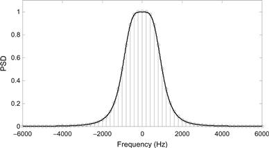
Figure 12.6 A comparison of the exact PSD along with the discrete approximation for Example 12.4. (For color verssion of this figure, the reader is referred to web verssion of this chapter.)

Figure 12.7 A realization of the random process of Example 12.4.


12.2.2 Time Domain Approach
A simple alternative to the previous frequency domain approach is to perform time domain filtering on a white Gaussian noise process as illustrated in Figure 12.8. Suppose white Gaussian noise with PSD, SXX (f) = 1 is input to an LTI filter that can be described by the transfer function, H(f). Then, from the results in Chapter 11, it is known that the PSD of the output process is SYY (f) = |H(f)|2. Therefore, in order to create a Gaussian random process, Y(t), with a prescribed PSD, SYY (f), we can construct a white process and pass this process through an appropriately designed filter. The filter should have a magnitude response which satisfies
![]() 12.12
12.12
![]()
Figure 12.8 Time domain filtering to create a colored Gaussian random process.
The phase response of the filter is irrelevant, and hence, any convenient phase response can be given to the filter.
This technique is particularly convenient when the prescribed PSD, SYY (f), can be written as the ratio of two polynomials in f. Then the appropriate transfer function can be found through spectral factorization techniques. If the desired PSD is a more complicated function of f, then designing and/or implementing a filter to produce that PSD may be difficult. In that case, it may be necessary to use an approximate filter design.
Example 12.5
In this example, we design the filter needed to generate the random process specified in Example 12.4 using the time domain method. The PSD is factored as follows:

If the first two poles are associated with H(f) (and the last two with H*(f)), then the filter has a transfer function of

which can be represented in the time domain as
![]()
where ![]() . For the purposes of creating a random process with the desired spectrum, the negative sign in front of this impulse response is irrelevant and can be ignored. Therefore, to produce the desired random process, we start by generating a white Gaussian random process and then convolve the input with the impulse response specified above.
. For the purposes of creating a random process with the desired spectrum, the negative sign in front of this impulse response is irrelevant and can be ignored. Therefore, to produce the desired random process, we start by generating a white Gaussian random process and then convolve the input with the impulse response specified above.
Once an appropriate analog filter has been designed, the filter must be converted to a discrete time form. If the sampling rate is taken to be sufficiently high, then the impulse response of the discrete time filter can be found by simply sampling the impulse response of the continuous time filter. This is the so-called impulse invariance transformation. However, because of aliasing that occurs in the process of sampling the impulse response, the frequency response of the digital filter will not be identical to that of the original analog filter unless the analog filter is absolutely bandlimited. Of course, if the analog filter is approximately bandlimited and if the sampling rate is sufficiently large, this aliasing can be kept to a minimum and the resulting digital filter will produce a very good approximation to the desired frequency response.
An alternative popular approach for producing a digital filter from an analog design is to use a bilinear transformation. That is, suppose we have an analog filter with transfer function Ha (s). A digital approximation to this filter, Hd (z), can be obtained (assuming a sampling frequency of fs) according to
![]() 12.13
12.13
One advantage of the bilinear transformation is that if the analog filter is stable, then the digital filter will be stable as well. Note also that if the analog filter is an nth order filter, then the order of the digital filter will be no more than n as well.
Example 12.6
In this example, we find the digital approximation to the analog filter designed in Example 12.5 using the bilinear approximation. From the results of that example, the analog filter was a second-order Butterworth filter whose transfer function (in terms of s) was given by

where ![]() is the 3-dB frequency of the filter in radians per second. After a little bit of algebraic manipulation, application of the bilinear transformation in Equation (12.13) results in
is the 3-dB frequency of the filter in radians per second. After a little bit of algebraic manipulation, application of the bilinear transformation in Equation (12.13) results in
![]()
where ![]() and Γ = fs
/(πf3). Figure 12.9 shows a plot of the impulse response of this filter as well as one realization of the random process created by passing white Gaussian noise through this filter. Note that for this example, the impulse response of the filter lasts for about 1 ms (this makes sense since the bandwidth was 1 kHz). Therefore, when creating the filtered process, at least the first millisecond of output data should be discarded since the contents of the digital filter have not reached a statistical steady state until that point. The relevant MATLAB code follows
and Γ = fs
/(πf3). Figure 12.9 shows a plot of the impulse response of this filter as well as one realization of the random process created by passing white Gaussian noise through this filter. Note that for this example, the impulse response of the filter lasts for about 1 ms (this makes sense since the bandwidth was 1 kHz). Therefore, when creating the filtered process, at least the first millisecond of output data should be discarded since the contents of the digital filter have not reached a statistical steady state until that point. The relevant MATLAB code follows

Figure 12.9 (a) Impulse response and (b) a single realization of the output of the filter designed in Example 12.6.

One advantage of the time domain approach is that it is convenient for generating very long realizations of the random process. Once the filter is designed, the output process is created by performing a convolution of the impulse response of the filter with a white input sequence. The complexity of this operation is linear in the length of the sequence. Furthermore, the process of creating a long sequence can be broken into several smaller sequences. The smaller sequences can then be concatenated together to create a long sequence. There will be no discontinuities at the points of concatenation if the contents of the filter are stored after each realization and used as the starting contents for the next realization.
Some care must be taken when using the time domain method if the desired sampling rate of the process is much larger than the bandwidth of the filter. In this case, the poles of the digital filter will be close to the unit circle and the filter might exhibit stability problems. This is illustrated in Figure 12.10 where the magnitude of the poles of the digital filter from Example 12.6 is plotted as a function of the sampling rate. Note that when the rate at which the process is sampled becomes a few hundred times the bandwidth of the filter, the poles of the digital filter become very close to the unit circle. This problem can easily be avoided by creating a digital filter to create samples of the process at a lower rate (perhaps at several times the bandwidth of the filter so as to avoid aliasing) and then upsampling (through interpolation) the resulting process to any desired rate.

Figure 12.10 Magnitude of the filter poles as a function of sampling frequency for the filter designed in Example 12.6.
12.2.3 Generation of Gaussian White Noise
Generation of a white noise process is exceedingly common and also is very simple. However, it is often the source of frequent mistakes among engineers, so we felt it worth making a few comments about computer generation of white Gaussian noise processes. The source of confusion in the generation of white noise is that one cannot represent white noise from its time domain samples. White noise has infinite power; therefore, samples of a white noise process would require infinite variance. Alternatively, white noise has infinite bandwidth, so the Nyquist rate for recovering white noise from its samples would be infinite. In order to represent a “white” process in discrete time, we must invoke some form of prefiltering before sampling. This will limit the bandwidth so that a finite sampling rate can be used, and at the same time, it will limit the power of the process so that the resulting samples of the filtered white process will have a finite variance.
Strictly speaking, once we filter the white noise it is no longer white, but this should not be of too much concern. In practice, there is no such thing as truly white noise. Recall that the white noise model was an approximation to a noise process which had a constant PSD over a very large (but not infinite) bandwidth. Furthermore, any equipment we use to measure or receive the noise will automatically filter the process. With this in mind, we imagine a prefilter that has a bandwidth that is much larger than any bandwidth we are concerned with in the specific system we are simulating. The noise we create, although not truly white, will behave as though it were white for all practical purposes.
In order to simplify the process of creating the samples of the prefiltered white noise, it is common to employ an ideal lowpass prefilter with bandwidth W as illustrated in Figure 12.11. Now that the process is bandlimited, it can be represented by samples at any rate that satisfies fs ≥ 2 W. Since the prefilter is ideal, the autocorrelation function of the filter output is easily calculated to be

Figure 12.11 A/D conversion process for white noise.
![]() 12.14
12.14
Note that since this sinc function has nulls at multiples of 1/2 W, the samples of the filtered process will be uncorrelated provided that the samples are spaced by any integer multiple of 1/2 W. In other words, if the sampling rate satisfies fs = 2 W/n for any integer n, then the samples of the prefiltered white noise will be uncorrelated. By choosing n = 1 so that the sampling rate is exactly the Nyquist rate, fs = 2 W, the process can be recovered from the discrete samples and the samples are uncorrelated. For Gaussian noise, this implies that the filtered white noise can be represented by a sequence of independent, zero-mean, Gaussian random variables with variance of σ2 = No W. Note that the variance of the samples and the rate at which they are taken are related by σ2 = No fs /2.
The lesson to be learned here is that if we wish to represent Gaussian white noise as a sequence of independent Gaussian random variables, then there is an implicit assumption about the nature of the prefiltering. Furthermore, to be consistent with this assumption, the variance of the samples must be adjusted when the sampling rate is changed. The variance and sampling rate cannot be selected independently.
12.3 Simulation of Rare Events
Quite often, we are interested in estimating the probability of some event, A. If analytically calculating this probability is too cumbersome, we can design a computer program to simulate the system in question and then observe whether or not the event occurs. By repeating this procedure many times, we can observe how often the event A occurs and hence get an estimate of its probability through a relative frequency approach. The event A could be a bit error in a digital communications system—in which case we are interested in calculating bit error probability—or it could be a buffer overflow in a computer network or even something as extravagant as breaking the bank at the blackjack table.
12.3.1 Monte Carlo Simulations
In general, suppose we have the ability to recreate (simulate) the experiment an arbitrary number of times and define a sequence of Bernoulli random variables, Xi , that are defined according to
 12.15
12.15
Hence, Xi is simply an indicator function for the event A. If the experiments are independent, then the probability of the event A, pA , can be estimated according to
 12.16
12.16
This is nothing more than estimating the mean of an IID sequence of random variables. From the development of Chapter 7, we know that this estimator is unbiased and that as n → ∞ the estimate converges (almost everywhere via the strong law of large numbers) to the true probability.
In practice, we do not have the patience to run our simulation an infinite number of times nor do we need to. At some point, the accuracy of our estimate should be “good enough,” but how many trials is enough? Some very concrete answers to this question can be obtained using the theory developed in Chapter 7. If the event A is fairly probable, then it will not take too many trials to get a good estimate of the probability, in which case runtime of the simulation is not really too much of an issue. However, if the event A is rare, then we will need to run many trials to get a good estimate of pA. In the case when n gets large, we want to be sure not to make it any larger than necessary so that our simulation runtimes do not get excessive. Thus, the question of how many trials to run becomes important when simulating rare events.
Assuming n is large, the random variable ![]() A can be approximated as a Gaussian random variable via the central limit theorem. The mean and variance are E[
A can be approximated as a Gaussian random variable via the central limit theorem. The mean and variance are E[![]() A
] = pA
and
A
] = pA
and ![]() , respectively. One can then set up a confidence interval based on the desired accuracy. For example, suppose we wish to obtain an estimate that is within 1% of the true value with 90% probability. That is, we want to run enough trials to insure that
, respectively. One can then set up a confidence interval based on the desired accuracy. For example, suppose we wish to obtain an estimate that is within 1% of the true value with 90% probability. That is, we want to run enough trials to insure that
![]() 12.17
12.17
From the results of Chapter 7, Section 7.5, we get
 12.18
12.18
where the value of c0.1 is taken from Table 7.1 as c0.1 = 1.64. Solving for n gives us an answer for how long to run the simulation:
![]() 12.19
12.19
Or in general, if we want the estimate, ![]() A
, to be within β percent of the true value (i.e.,
A
, to be within β percent of the true value (i.e., ![]() with probability α, then the number of trials in the simulation should be chosen according to
with probability α, then the number of trials in the simulation should be chosen according to
 12.20
12.20
This result is somewhat unfortunate because in order to know how long to run the simulation, we have to know the value of the probability we are trying to estimate in the first place. In practice, we may have a crude idea of what to expect for pA which we could then use to guide us in selecting the number of trials in the simulation. However, we can use this result to give us very specific guidance in how to choose the number of trials to run, even when pA is completely unknown to us. Define the random variable NA to be the number of occurrences of the event A in n trials, that is,
![]() 12.21
12.21
Note that E[NA ] = npA . That is, the quantity npA can be interpreted as the expected number of occurrences of the event A in n trials. Multiplying both sides of Equation (12.20) by pA then produces
![]() 12.22
12.22
Hence, one possible procedure to determine how many trials to run is to repeat the experiment for a random number of trials until the event A occurs some fixed number of times as specified by Equation (12.22). Let Mk be the random variable which represents the trial number of the kth occurrence of the event A. Then, one could form an estimate of pA according to
![]() 12.23
12.23
It turns out that this produces a biased estimate; however, a slightly modified form,
![]() 12.24
12.24
produces an unbiased estimate (see Exercise 7.12).
Example 12.7
Suppose we wish to estimate the probability of an event that we expect to be roughly on the order of p ~ 10−4. Assuming we want 1% accuracy with a 90 % confidence level, the number of trials needed will be
![]()
Alternatively, we need to repeat the simulation experiment until we observe the event
![]()
times. Assuming we do not have enough time available to repeat our simulation over 1/4 of a billion times, we would have to accept less accuracy. Suppose that due to time limitations we decide that we can only repeat our experiment 1 million times, then we can be sure that with 90% confidence, the estimate will be within the interval (p − ε, p + ε), if ε is chosen according to

With 1 million trials we can only be 90% sure that the estimate is within 16.4% of the true value.
The preceding example demonstrates that using the Monte Carlo approach to simulating rare events can be very time consuming in that we may need to repeat our simulation experiments many times to get a high degree of accuracy. If our simulations are complicated, this may put a serious strain on our computational resources. The next subsection presents a novel technique, which when applied intelligently can substantially reduce the number of trials we may need to run.
12.3.2 Importance Sampling
The general idea behind importance sampling is fairly simple. In the Monte Carlo approach, we spend a large amount of time with many repetitions of an experiment while we are waiting for an event to occur which may happen only very rarely. In importance sampling, we skew the distribution of the underlying randomness in our experiment so that the “important” events happen more frequently. We can then use analytical tools to convert our distorted simulation results into an unbiased estimate of the probability of the event in which we are interested. To help present this technique, we first generalize the problem treated in Section 12.3.1. Suppose the simulation experiment consisted of creating a sequence of random variables, X = (X1, X2, …, Xm ) according to some density, fX (x), and then observing whether or not some event A occurred which could be defined in terms of the Xi . For example, suppose Xi represents the number of messages that arrive at a certain node in a computer communications network at time instant i. Furthermore, suppose that it is known that the node requires a fixed amount of time to forward each message along to its intended destination and that the node has some finite buffer capacity for storing messages. The event A might represent the event that the node’s buffer overflows, and thus a message is lost during the time interval i = 1, 2, …, m. Ideally, the communication network has been designed so that this event is fairly uncommon, but it is desirable to quantify how often this overflow will occur. While it may be fairly straightforward to determine whether or not a buffer overflow has occurred given a specific sequence of arrivals, X = x, determining analytically the probability of buffer overflow may be difficult, so we decide to approach this via simulation. Let ηA (X) be an indicator function for the event A. That is, let ηA (x) = 1 if x is such that the event A occurs and ηA (x) = 0 otherwise. Also, let x(i) be the realization of the random vector X that occurs on the ith trial of the simulation experiment. Then the Monte Carlo approach to estimating pA is
 12.25
12.25
Now suppose instead we generate a sequence of random variables Y = (Y1, Y2, …, Ym ) according to a different distribution f Y (y) and form the estimate
 12.26
12.26
It is pretty straightforward (see Exercise 12.11) to establish that this estimator is also unbiased. By carefully choosing the density function, f Y (y), we may be able to drastically speed up the convergence of the series in Equation (12.26) relative to that in Equation (12.25).
The important step here is to decide how to choose the distribution of Y. In general, the idea is to choose a distribution of Y so that the event {ηA (Y) = 1} occurs more frequently than the event {ηA (X) =1}. In other words, we want to choose a distribution so that the “important” event is sampled more often. It is common to employ the so-called twisted distribution, which calls on concepts taken from large deviation theory. But using these techniques is beyond the scope of this book. Instead, we take an admittedly ad hoc approach here and on a case-by-case basis we try to find a good (but not necessarily optimal) distribution. An example of using importance sampling is provided in the following application section.
12.4 Engineering Application: Simulation of a Coded Digital Communication System
In this section, we demonstrate use of the importance sampling technique outlined in the previous section in the simulation of a digital communication system with convolutional coding. A basic block diagram of the system is illustrated in Figure 12.12. A source outputs binary data, Xi , which is input to an encoder that adds redundancy to the data stream for the purposes of error protection. For this particular example, an encoder with a code rate of 1/2 is used. Simply put, this means that for every one bit input, the convolutional encoder outputs two coded bits, {Y2i −1, Y2i }. To keep this example simple, the channel is modeled as one which randomly inverts bits with some probability p in a memoryless fashion. That is, what happens to one bit on the channel is independent of any of the other bits. Given a vector of bits input to the channel, Y = (Y1, Y2, …, Yn ), the probability of observing a certain output of the channel R = (R1, R2, …, Rn ) is given by

Figure 12.12 Block diagram of a digital communication system.
 12.27
12.27
where
 12.28
12.28
The decoder then takes the received sequence output from the channel and determines what was the most likely data sequence.
For this example, it is not necessary to understand the workings of the encoder and decoder. We will just assume the existence of some computer subroutines which simulate their functions. Each trial of our simulation experiment will consist of randomly generating an IID sequence of equally likely data bits, passing them through the encoder, randomly corrupting some of the encoded bits according to the channel model we have developed, and then decoding the received sequence. The decoded bits are then compared with the original bits to measure the decoded bit error probability. For the purposes of this example, it is assumed that data are transmitted in blocks of 50 information bits (which are encoded into blocks of 100 coded bits). We refer to each of these blocks as a frame. The channel is simulated by creating an error pattern E = (E1, E2, …,E100) where the Ei are a sequence of IID random variables with Pr(Ei -=1) = p and Pr(Ei = 0) = 1− p. Then
![]() 12.29
12.29
The event {Ei= 1} implies that the i th bit is inverted in the process of going through the channel while {Ei = 0} means that the ith bit is received correctly.
Using the standard Monte Carlo approach, the decoded bit error rate is estimated according to
![]() 12.30
12.30
where m is the number of packets transmitted in the simulation; n is the number of bits per packet; and the function η![]() counts the number of bit errors that occurred in the j th packet. If the channel error rate, p, is fairly high (e.g., a noisy channel), then the Monte Carlo approach will work quite nicely. However, if p « 1, then channel errors will be infrequent and the decoder will usually correct them. Thus, the decoded error probability will be very small and the Monte Carlo approach will require us to simulate an astronomical number of packets.
counts the number of bit errors that occurred in the j th packet. If the channel error rate, p, is fairly high (e.g., a noisy channel), then the Monte Carlo approach will work quite nicely. However, if p « 1, then channel errors will be infrequent and the decoder will usually correct them. Thus, the decoded error probability will be very small and the Monte Carlo approach will require us to simulate an astronomical number of packets.
Alternatively, consider a simple importance sampling approach. To avoid simulating endless packets which ultimately end up error free, we now create IID error patterns with Pr(Ei = 1) = q, where q is some suitably chosen value which is larger than p. Note that any pattern e = (e1, e2, …, e100) that contains exactly w 1s and 100 − w zeros will be generated with probability Pr(e) = qw (1− q)100−w. Let w(e) be the number of 1s in a particular error pattern, e. Then, our importance sampling estimate of the decoded error probability will be
![]() 12.31
12.31
Simulation results are shown in Figure 12.13 where the channel bit error probability is p = 0.01. Note that there are theoretical bounds that tell us that for this example, the actual probability of decoded bit error should be bounded by 1.97 × 10⁻⁵ ≤ Pe ≤ 6.84 × 10⁻⁵. To get fairly accurate results via the Monte Carlo approach, we would expect to have to simulate on the order of several hundred thousand packets. It is seen in Figure 12.13 that indeed, even after simulating 10,000 packets, the estimated error probability has still not converged well. For the importance sampling results, we used q = 0.05 so that important error events occurred much more frequently. As seen in the figure, the estimated error probability has converged rather nicely after simulating only a few thousand packets. Therefore, for this example, using the importance sampling method has sped up the simulation time by a few orders of magnitude.

Figure 12.13 Simulation results for a coded digital communication system using standard Monte Carlo and importance sampling techniques.
Exercises
Section 12.1: Computer Generation of Random Variables
12.1 Consider the periodic sequence generated by the four-stage shift register in Figure 12.1. Suppose the sequence is converted to ± 1-valued sequence by mapping all 1’s to −1’s and all 0’s to 1’s. One period of the resulting sequence is:
![]()
Calculate the autocorrelation function of this periodic sequence. Note: Do not just treat this sequence as having finite length. The sequence is infinite in both directions. The finite sequence shown above is just one period of the infinite periodic sequence.
12.2 Sketch the shift register described by the octal number 75. Find the sequence output by this shift register assuming that the shift register is initially loaded with all ones.
12.3 A certain N-stage shift register has its tap connections configured so that it produces an m-sequence. The shift register is initially loaded with the contents c = (c0, cl, …, CN− 1) resulting in a periodic sequence of period 2N − 1. Prove that if the shift register is loaded with some other contents c′ ≠ 0, the new output sequence will be a cyclic shift of the original output sequence. Hint: Recall that for an m-sequence, the shift register must cycle through all nonzero states.
12.4 Suppose we create a binary ± 1-valued sequence of length N by drawing N independent realizations of a Bernoulli random variable to form one period of the sequence. Compute the autocorrelation function of this random Bernoulli sequence.
12.5 Suppose a pseudorandom sequence is constructed using the power residue method as described by
![]()
Find the period and the sequence which results for the following values of (a, q). For each case, assume the seed is xo
= 1.
12.6 Suppose a pseudorandom sequence is constructed using the power residue method as discussed in Exercise 12.5. If q = 11, find a value of a that leads to a sequence with maximum possible period.
12.7 Find a transformation which will change a uniform random variable into each of the following distributions (see Appendix D for the definitions of these distributions if necessary):
Section 12.2: Generation of Random Processes
12.8 Suppose we wish to generate a 10-ms realization of a zero-mean Gaussian random process with a PSD of
![]()
(a) Find the bandwidth that contains 99 % of the total power in the random process.
(b) Determine how many frequency samples are needed for the frequency domain method described in Section 12.2.1.
12.9 Suppose we wanted to generate the random process whose PSD is given in Exercise 12.8 using the time domain method discussed in Section 12.2.2.
(a) Find the transfer function of the analog filter which will produce the desired output PSD when the input is a zero-mean, white Gaussian random process.
(b) Use a bilinear transformation to convert the analog filter to a digital filter.
(c) What is the approximate duration of the impulse response of the digital filter if the 3-dB frequency of the random process is f3 = 1kHz.
12.10 Suppose a zero-mean Gaussian random process, X(t), has a PSD given by
![]()
where fo= 1 kHz. We desire to simulate a 5-ms segment of this process sampled at a rate of 2 kHz. Therefore, 10 samples will need to be created in our simulation. We will create the samples of the process by first generating 10 uncorrelated Gaussian random variables and then pass those variables through an appropriate transformation matrix, A.
Section 12.3: Simulation of Rare Events
12.11 Suppose we use a Monte Carlo simulation approach to simulate the probability of some rare event A. It is decided that we will repeat the simulation until the event A occurs 35 times. With what accuracy will we estimate PA to within a 90% confidence level?
12.12 Prove that the importance sampling (IS) estimator of Equation (12.26) is unbiased. That is, show that
![]()
12.13 Show that the variance of the IS estimator of Equation (12.26) is given by
12.14 Suppose the random variable X has an exponential distribution, fX
(x) = exp (−x) u (x). We wish to estimate the probability of the event A = {X > xo
} via simulation. We will compare the standard Monte Carlo estimate,

where the random variables Xi
are chosen according to the exponential distribution specifed by PDF fX
(x), with an importance sampling estimate,

where the random variables Yi are chosen from a suitable distribution specified by its PDF, fY (y). Note that both estimators are unbiased, so we will compare these estimators by examining their variances.
(a) Find the variance of the Monte Carlo estimate.
(b) Find the variance of the IS estimator assuming that the random variables Yi are chosen from a scaled exponential distribution, fY (y) = aexp (−ay) u (y).
(c) Assuming that xo = 20, find the value of a that minimizes the variance of the IS estimator using the scale exponential distribution.
(d) How much faster do you expect the IS simulation to run as compared to the MC simulation?
12.15 Repeat Exercise 12.14 using random variables X that follow a Gaussian distribution fX (x) = exp (−x2/2). Also, for parts (b)−(d) use a shifted distribution for the importance sampling estimator of the form fY (y) = exp (−(x − a)2/2). Also, for this problem, use xo = 6.
MATLAB Exercises
12.16 We wish to generate a periodic sequence of numbers that cycles through the integers from 1 to 100 in a pseudorandom fashion. Choose a pair of integers (a, q) that can be used in the power residue method to produce a sequence of the desired form. Write a MATLAB program to verify that the sequence produced does in fact cycle through each of the integers 1−100 exactly once each before the sequence repeats.
12.17 Let X~ N(2, 1), Y ~ N(0, 1), Z ~ N(0, 1), and W = ![]() . We desire to find Pr(W > 3). Write a MATLAB program to estimate this probability through Monte Carlo simulation techniques. If we want to be 90% sure that our estimate is within 5 % of the true value, about how many times should we observe the event {W > 3}? Run your program and provide the estimate of the desired probability. Can you find the probability analytically?
. We desire to find Pr(W > 3). Write a MATLAB program to estimate this probability through Monte Carlo simulation techniques. If we want to be 90% sure that our estimate is within 5 % of the true value, about how many times should we observe the event {W > 3}? Run your program and provide the estimate of the desired probability. Can you find the probability analytically?
12.18 Write a MATLAB program to generate a realization of the random process from Exercise 12.8 (using the frequency domain method). Use a periodogram to estimate the PSD of the process using the realization of the process you generated. Does your PSD estimate agree with the PSD that the process is designed to possess?
12.19 Write a MATLAB program to generate a realization of the random process from Exercise 12.9 (using the time domain method). Use a periodogram to estimate the PSD of the process using the realization of the process you generated. Does your PSD estimate agree with the PSD that the process is designed to possess?