CHAPTER 2
Introduction to Probability Theory
Many electrical engineering students have studied, analyzed, and designed systems from the point of view of steady-state and transient signals using time domain or frequency domain techniques. However, these techniques do not provide a method for accounting for variability in the signal nor for unwanted disturbances such as interference and noise. We will see that the theory of probability and random processes is useful for modeling the uncertainty of various events (e.g., the arrival of telephone calls and the failure of electronic components). We also know that the performance of many systems is adversely affected by noise, which may often be present in the form of an undesired signal that degrades the performance of the system. Thus, it becomes necessary to design systems that can discriminate against noise and enhance a desired signal.
How do we distinguish between a deterministic signal or function and a stochastic or random phenomenon such as noise? Usually, noise is defined to be any undesired signal, which often occurs in the presence of a desired signal. This definition includes deterministic as well as non-deterministic signals. A deterministic signal is one which may be represented by some parameter values, such as a sinusoid, which may be perfectly reconstructed given an amplitude, frequency, and phase. Stochastic signals, such as noise, do not have this property. While they may be approximately represented by several parameters, stochastic signals have an element of randomness which prevent them from being perfectly reconstructed from a past history. As we saw in Chapter 1 (Figure 1.2), even the same word spoken by different speakers is not deterministic; there is variability, which can be modeled as a random fluctuation. Likewise, the amplitude and/or phase of a stochastic signal cannot be calculated for any specified future time instant even though the entire past history of the signal may be known. However, the amplitude and/or phase of a stochastic signal can be predicted to occur with a specified probability, provided certain factors are known. The theory of probability provides a tool to model and analyze phenomena that occur in many diverse fields, such as communications, signal processing, control, and computers. Perhaps the major reason for studying probability and random processes is to be able to model complex systems and phenomena.
2.1 Experiments, Sample Spaces, and Events
The relationship between probability and gambling has been known for some time. Over the years, some famous scientists and mathematicians have devoted time to probability: Galileo wrote on dice games; Laplace worked out the probabilities of some gambling games; and Pascal and Bernoulli, while studying games of chance, contributed to the basic theory of probability. Since the time of this early work, the theory of probability has become a highly developed branch of mathematics. Throughout these beginning sections on basic probability theory, we will often use games of chance to illustrate basic ideas that will form the foundation for more advanced concepts. To start with, a few simple definitions are presented.
Definition 2.1: An experiment is a procedure we perform (quite often hypothetical) that produces some result. Often the letter E is used to designate an experiment (e.g., the experiment E5 might consist of tossing a coin five times).
Definition 2.2: An outcome is a possible result of an experiment. The Greek letter xi (ξ;) is often used to represent outcomes (e.g., the outcome ξ;1 of experiment E5 might represent the sequence of tosses heads-heads-tails-heads-tails; however, the more concise HHTHT might also be used).
Definition 2.3: An event is a certain set of outcomes of an experiment (e.g., the event C associated with experiment E5 might be C = {all outcomes consisting of an even number of heads}).
Definition 2.4: The sample space is the collection or set of “all possible” distinct (collectively exhaustive and mutually exclusive) outcomes of an experiment. The letter S is used to designate the sample space, which is the universal set of outcomes of an experiment. A sample space is called discrete if it is a finite or a countably infinite set. It is called continuous or a continuum otherwise.
The reason we have placed quotes about the words all possible in Definition 2.4 is explained by the following imaginary situation. Suppose we conduct the experiment of tossing a coin. While it is conceivable that the coin may land on edge, experience has shown us that such a result is highly unlikely to occur. Therefore, our sample space for such experiments typically excludes such unlikely outcomes. We also require, for the present, that all outcomes be distinct. Consequently, we are considering only the set of simple outcomes that are collectively exhaustive and mutually exclusive.
Example 2.1
Consider the example of flipping a fair coin once, where fair means that the coin is not biased in weight to a particular side. There are two possible outcomes, namely, a head or a tail. Thus, the sample space, S, consists of two outcomes, ξ;1 = H to indicate that the outcome of the coin toss was heads, and ξ;2 = T to indicate that the outcome of the coin toss was tails.
Example 2.2
A cubical die with numbered faces is rolled and the result observed. The sample space consists of six possible outcomes ξ;1 = 1, ξ;2 = 2, …, ξ;6 = 6, indicating the possible faces of the cubical die that may be observed.
Example 2.3
As a third example, consider the experiment of rolling two dice and observing the results. The sample space consists of 36 outcomes, which may be labeled by the ordered pairs ξ;1 = (1, 1), ξ;2 = (1, 2), ξ;3 = (1, 3), …, ξ;6 = (1, 6), ξ;7 = (2, 1), ξ;8 = (2, 2), …, ξ;36 = (6, 6); the first component in the ordered pair indicates the result of the toss of the first die and the second component indicates the result of the toss of the second die. Many events can be defined from this experiment, such as:
A = {the sum of the outcomes of the two rolls = 4},
B = {the outcomes of the two rolls are identical},
C = {the first roll was bigger than the second}.
An alternative way to consider this experiment is to imagine that we conduct two distinct experiments, with each consisting of rolling a single die. The sample spaces (S1 and S2) for each of the two experiments are identical, namely, the same as Example 2.2. We may now consider the sample space, S, of the original experiment to be the combination of the sample spaces, S1 and S2, which consist of all possible combinations of the elements of both S1 and S2. This is an example of a combined sample space.
Example 2.4
For our fourth experiment, let us flip a coin until a tails occurs. The experiment is then terminated. The sample space consists of a collection of sequences of coin tosses. Label these outcomes as ξ; n , n = 1, 2, 3, …. The final toss in any particular sequence is a tail and terminates the sequence. The preceding tosses prior to the occurrence of the tail must be heads. The possible outcomes that may occur are:
ξ;1 = (T), ξ;2 = (H, T), ξ;3 = (H, H, T),….
Note that in this case, n can extend to infinity. This is another example of a combined sample space resulting from conducting independent, but identical experiments. In this example, the sample space is countably infinite, while the previous sample spaces were finite.
Example 2.5
As a last example, consider a random number generator which selects a number in an arbitrary manner from the semi-closed interval [0, 1). The sample space consists of all real numbers, x, for which 0 ≤ x ≤ 1. This is an example of an experiment with a continuous sample space. We can define events on a continuous space as well, such as:
Other examples of experiments with continuous sample spaces include the measurement of the voltage of thermal noise in a resistor or the measurement of the (x, y, z) position of an oxygen molecule in the atmosphere. Examples 2.1-2.4 illustrate discrete sample spaces.
There are also infinite sets that are uncountable and that are not continuous, but these sets are beyond the scope of this book. So for our purposes, we will consider only the preceding two types of sample spaces. It is also possible to have a sample space that is a mixture of discrete and continuous sample spaces. For the remainder of this chapter, we shall restrict ourselves to the study of discrete sample spaces.
A particular experiment can often be represented by more than one sample space. The choice of a particular sample space depends upon the questions that are to be answered concerning the experiment. This is perhaps best explained by recalling Example 2.3 in which a pair of dice was rolled. Suppose we were asked to record after each roll the sum of the numbers shown on the two faces. Then, the sample space could be represented by only eleven outcomes, ξ;1 = 2, ξ;2 = 3, ξ;3 = 4, …, ξ;11 = 12. However, the original sample space is in some way, more fundamental, since the sum of the die faces can be determined from the numbers on the die faces. If the second representation is used, it is not sufficient to specify the sequence of numbers that occurred from the sum of the numbers.
2.2 Axioms of Probability
Now that the concepts of experiments, outcomes, and events have been introduced, the next step is to assign probabilities to various outcomes and events. This requires a careful definition of probability. The words probability and probable are commonly used in everyday language. The meteorologist on the evening news may say that rain is probable for tomorrow or he may be more specific and state that the chance (or probability) of rain is 70%. Although this sounds like a precise statement, we could interpret it in several ways. Perhaps, it means that about 70% of the listening audience will experience rain. Or, maybe if tomorrow could be repeated many times, 70% of the tomorrows would have rain while the other 30% would not. Of course, tomorrow cannot be repeated and this experiment can only be run once. The outcome will be either rain or no rain. The meteorologist may like this interpretation since there is no way to repeat the experiment enough times to test the accuracy of the prediction. However, there is a similar interpretation that can be tested. We might say that any time a day with similar meteorological conditions presents itself, the following day will have rain 70% of the time. In fact, it may be his or her past experience with the given weather conditions that led the meteorologist to the prediction of a 70% chance of rain.
It should be clear from our everyday usage of the word probability that it is a measure of the likelihood of various events. So in general terms, probability is a function of an event that produces a numerical quantity that measures the likelihood of that event. There are many ways to define such a function, which we could then call probability. In fact, we will find several ways to assign probabilities to various events, depending on the situation. Before we do that, however, we start with three axioms that any method for assigning probabilities must satisfy:
Axiom 2.1: For any event A, Pr(A) ≥ 0 (a negative probability does not make sense).
Axiom 2.2: If S is the sample space for a given experiment, Pr(S) = 1 (probabilities are normalized so that the maximum value is unity).
Axiom 2.3a: If A ∩ B = Ø, then Pr(A ∪ B) = Pr(A) + Pr(B).
As the word axiom implies, these statements are taken to be self-evident and require no proof. In fact, the first two axioms are really more of a self-imposed convention. We could have allowed for probabilities to be negative or we could have normalized the maximum probability to be something other than one. However, this would have greatly confused the subject and we do not consider these possibilities. From these axioms (plus one more to be presented shortly), the entire theory of probability can be developed. Before moving on to that task, a corollary to Axiom 2.3a is given.
Corollary 2.1: Consider M sets A1, A2, …, AM which are mutually exclusive, Ai ∩ Aj = Ø for all i ≠ j,
 (2.1)
(2.1)
Proof: This statement can be proven using mathematical induction. For those students who are unfamiliar with this concept, the idea behind induction is to show that if the statement is true for M = m, then it must also hold for M = m + 1. Once this is established, it is noted that by Axiom 2.3a, the statement applies for M = 2, and hence it must be true for M = 3. Since it is true for M = 3, it must also be true for M = 4, and so on. In this way, we can prove that Corollary 2.1 is true for any finite M. The details of this proof are left as an exercise for the reader (see Exercise 2.7).
Unfortunately, the proof just outlined is not sufficient to show that Corollary 2.1 is true for the case of an infinite number of sets. That has to be accepted on faith and is listed here as the second part of Axiom 2.3.
Axiom 2.3b: For an infinite number of mutually exclusive sets, Ai , i = 1, 2, 3 …, Ai ∩ Aj = Ø for all i ≠ j,
 (2.2)
(2.2)
It should be noted that Axiom 2.3a and Corollary 2.1 could be viewed as special cases of Axiom 2.3b. So, a more concise development could be obtained by starting with Axioms 2.1, 2.2, and 2.3b. This may be more pleasing to some, but we believe the approach given here is little easier to follow for the student learning the material for the first time.
The preceding axioms do not tell us directly how to deal with the probability of the union of two sets that are not mutually exclusive. This can be determined from these axioms as is now shown.
Theorem 2.1: For any sets A and B (not necessarily mutually exclusive),
![]() (2.3)
(2.3)
Proof: We give a visual proof of this important result using the Venn diagram shown in Figure 2.1. To aid the student in the type of reasoning needed to complete proofs of this type, it is helpful to think of a pile of sand lying in the sample space shown in Figure 2.1. The probability of the event A would then be analogous to the mass of that subset of the sand pile that is above the region A and likewise for the probability of the event B. For the union of the two events, if we simply added the mass of the sand above A to the mass of the sand above B, we would double count that region which is common to both sets. Hence, it is necessary to subtract the probability of A ∩ B. We freely admit that this proof is not very rigorous. It is possible to prove Theorem 2.1 without having to call on our sand analogy or even the use of Venn diagrams. The logic of the proof will closely follow what we have done here. The reader is led through that proof in Exercise 2.8.

Figure 2.1 Venn diagram for proof of Theorem 2.1.
Many other fundamental results can also be obtained from the basic axioms of probability. A few simple ones are presented here. More will be developed later in this chapter and in subsequent chapters. As with Theorem 2.1, it might help the student to visualize these proofs by drawing a Venn diagram.
Theorem 2.2: ![]() .
.
Proof: 
![]()
Theorem 2.3: If A ⊂ B, then Pr(A) ≤ Pr(B).
Proof: See Exercise 2.10. ![]()
2.3 Assigning Probabilities
In the previous section, probability was defined as a measure of the likelihood of an event or of events which satisfyAxioms 2.1–2.3. How probabilities are assigned to particular events was not specified. Mathematically, any assignment that satisfies the given axioms is acceptable. Practically speaking, we would like to assign probabilities to events in such a way that the probability assignment actually represents the likelihood of occurrence of that event. Two techniques are typically used for this purpose and are described in the following paragraphs.
In many experiments, it is possible to specify all of the outcomes of the experiment in terms of some fundamental outcomes which we refer to as atomic outcomes. These are the most basic events that cannot be decomposed into simpler events. From these atomic outcomes, we can build more complicated and more interesting events. Quite often we can justify assigning equal probabilities to all atomic outcomes in an experiment. In that case, if there are M mutually exclusive exhaustive atomic events, then each one should be assigned a probability of 1/M. Not only does this make perfect common sense, it also satisfies the mathematical requirements of the three axioms which define probability. To see this, we label the M atomic outcomes of an experiment E as ξ; 1 , ξ;2, …, ξ;M . These atomic events are taken to be mutually exclusive and exhaustive. That is, ξ;i ∩ ξ;j = Ø for all i ≠ j, and ξ; 1 ∪ ξ; 2 ∪ … ∪ ξ; M = S. Then by Corollary 2.1 and Axiom 2.2,
![]() (2.4)
(2.4)
If each atomic outcome is to be equally probable, then we must assign each a probability of Pr(ξ; i ) = 1/M for there to be equality in the preceding equation. Once the probabilities of these outcomes are assigned, the probabilities of some more complicated events can be determined according to the rules set forth in Section 2.2. This approach to assigning probabilities is referred to as the classical approach.
Example 2.6
The simplest example of this procedure is the coin flipping experiment of Example 2.1. In this case, there are only two atomic events, ξ;1 = H and ξ;2 = T. Provided the coin is fair (again, not biased toward one side or the other), we have every reason to believe that these two events should be equally probable. These outcomes are mutually exclusive and collectively exhaustive (provided we rule out the possibility of the coin landing on end). According to our theory of probability, these events should be assigned probabilities of Pr(H) = Pr(T) = 1/2.
Example 2.7
Next consider the dice rolling experiment of Example 2.2. If the die is not loaded, the six possible faces of the cubicle die are reasonably taken to be equally likely to appear, in which case, the probability assignment is Pr(l) = Pr(2) = … = Pr(6) = 1/6. From this assignment, we can determine the probability of more complicated events, such as:
Example 2.8
In Example 2.3, a pair of dice were rolled. In this experiment, the most basic outcomes are the 36 different combinations of the six atomic outcomes of the previous example. Again, each of these atomic outcomes is assigned a probability of 1/36. Next, suppose we want to find the probability of the event A = {sum of two dice = 5}. Then,

Example 2.9
 In this example, we will use the MATLAB command rand to simulate the flipping of coins and the rolling of dice. The command rand (m, n) creates a matrix of m rows and n columns where each element of the matrix is a randomly selected number equally likely to fall anywhere in the interval (0, 1). By rounding this number to the nearest integer, we can create a randomly selected number equally likely to be 0 or 1. This can be used to simulate the flipping of a coin if we interpret 0 as “tails” and 1 as “heads” or vice versa. Similarly, if we multiply rand(1) by 6 and round up to the nearest integer, we will get one of the numbers 1, 2, …, 6 with equal probability. This can be used to simulate the rolling of a die. Try running the following script in MATLAB.
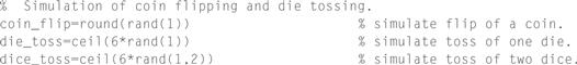
You should find that each time you run this script, you get different (random) looking results. With any MATLAB command, if you want more information on what the command does, type help followed by the command name at the MATLAB prompt for detailed information on that command. For example, to get help on the rand command, type help rand.
Care must be taken when using the classical approach to assigning probabilities. If we define the set of atomic outcomes incorrectly, unsatisfactory results may occur. In Example 2.8, we may be tempted to define the set of atomic outcomes as the different sums that can occur on the two dice faces. If we assign equally likely probability to each of these outcomes, then we arrive at the assignment
![]() (2.5)
(2.5)
Anyone with experience in games involving dice knows that the likelihood of rolling a 2 is much less than the likelihood of rolling a 7. The problem here is that the atomic events we have assigned are not the most basic outcomes and can be decomposed into simpler outcomes as demonstrated in Example 2.8.
This is not the only problem encountered in the classical approach. Suppose we consider an experiment that consists of measuring the height of an arbitrarily chosen student in your class and rounding that measurement to the nearest inch. The atomic outcomes of this experiment would consist of all the heights of the students in your class. However, it would not be reasonable to assign an equal probability to each height. Those heights corresponding to very tall or very short students would be expected to be less probable than those heights corresponding to a medium height. So, how then do we assign probabilities to these events? The problems associated with the classical approach to assigning probabilities can be overcome by using the relative frequency approach.
The relative frequency approach requires that the experiment we are concerned with be repeatable, in which case, the probability of an event, A, can be assigned by repeating the experiment a large number of times and observing how many times the event A actually occurred. If we let n be the number of times the experiment is repeated and nA the number of times the event A is observed, then the probability of the event A can be assigned according to
![]() (2.6)
(2.6)
This approach to assigning probability is based on experimental results and thus has a more practical flavor to it. It is left as an exercise for the reader (see Exercise 2.15) to confirm that this method does indeed satisfy the axioms of probability, and is thereby mathematically correct as well.
Example 2.10
Consider the dice rolling experiment of Examples 2.3 and 2.8. We will use the relative frequency approach to assign the probability of the event A = {sum of two dice = 5}. We simulated the tossing of two dice using the following MATLAB code. The results of this dice tossing simulation are shown in Table 2.1.
Table 2.1. Simulation of Dice Tossing Experiment


The next to last line of MATLAB code may need some explanation. The double equal sign asks MATLAB to compare the two quantities to see if they are equal. MATLAB responds with 1 for “yes” and 0 for “no.” Hence, the expression dice_sum==5 results in an n element vector where each element of the vector is either 0 or 1 depending on whether the corresponding element of dice_sum is equal to 5 or not. By summing all elements of this vector, we obtain the number of times the sum 5 occurs in n tosses of the dice.
To get an exact measure of the probability of an event, we must be able to repeat the event an infinite number of times—a serious drawback to this approach. In the dice rolling experiment of Example 2.8, even after rolling the dice 10,000 times, the probability of observing a 5 was measured to only two significant digits. Furthermore, many random phenomena in which we might be interested are not repeatable. The situation may occur only once, and therefore we cannot assign the probability according to the relative frequency approach.
2.4 Joint and Conditional Probabilities
Suppose that we have two events, A and B. We saw a few results in the previous section that dealt with how to calculate the probability of the union of two events, A ∪ B. At least as frequently, we are interested in calculating the probability of the intersection of two events, A ∩ B. This probability is referred to as the joint probability of the events A and B, Pr(A ∩ B). Usually, we will use the simpler notation Pr(A, B). This definition and notation extends to an arbitrary number of sets. The joint probability of the events, A1, A2, …, AM , is Pr(A1 ∩ A2 ∩ … ∩ AM ) and we use the simpler notation Pr(A1, A2, … AM ) to represent the same quantity.
Now that we have established what a joint probability is, how does one compute it? To start with, by comparing Axiom 2.3a and Theorem 2.1, it is clear that if A and B are mutually exclusive, then their joint probability is zero. This is intuitively pleasing, since if A and B are mutually exclusive, then Pr(A, B) = Pr(Ø), which we would expect to be zero. That is, an impossible event should never happen. Of course, this case is of rather limited interest, and we would be much more interested in calculating the joint probability of events that are not mutually exclusive.
In the general case when A and B are not necessarily mutually exclusive, how can we calculate the joint probability of A and B? From the general theory of probability, we can easily see two ways to accomplish this. First, we can use the classical approach. Both events A and B can be expressed in terms of atomic outcomes. We then write A ∩ B as the set of those atomic outcomes that are common to both and calculate the probabilities of each of these outcomes. Alternatively, we can use the relative frequency approach. Let nA, B be the number of times that A and B simultaneously occur in n trials. Then,
![]() (2.7)
(2.7)
Example 2.11
A standard deck of playing cards has 52 cards that can be divided in several manners. There are four suits (spades, hearts, diamonds and clubs) each of which has 13 cards (ace, 2, 3, 4, …, 10, jack, queen, king). There are two red suits (hearts and diamonds) and two black suits (spades and clubs). Also, the jacks, queens and kings are referred to as face cards, while the others are number cards. Suppose the cards are sufficiently shuffled (randomized) and one card is drawn from the deck. The experiment has 52 atomic outcomes corresponding to the 52 individual cards that could have been selected. Hence, each atomic outcome has a probability of 1/52. Define the events: A = {red card selected}, B = {number card selected}, and C = {heart selected}. Since the event A consists of 26 atomic outcomes (there are 26 red cards), then Pr(A) = 26/52 = 1/2. Likewise, Pr(B) = 40/52 = 10/13 and Pr(C) = 13/52 = 1/4. Events A and B have 20 outcomes in common, hence Pr(A, B) = 20/52 = 5/13. Likewise, Pr(A, C) = 13/52 = 1/4 and Pr(B, C) = 10/52 = 5/26. It is interesting to note that in this example, Pr(A, C) = Pr(C). This is because C ⊂ A and as a result A ∩ C = C.
Often the occurrence of one event may be dependent upon the occurrence of another. In the previous example, the event A = {a red card is selected} had a probability of Pr(A) = 1/2. If it is known that event C = {a heart is selected} has occurred, then the event A is now certain (probability equal to 1), since all cards in the heart suit are red. Likewise, if it is known that the event C did not occur, then there are 39 cards remaining, 13 of which are red (all the diamonds). Hence, the probability of event A in that case becomes 1/3. Clearly, the probability of event A depends on the occurrence of event C. We say that the probability of A is conditional on C, and the probability of A given knowledge that the event C has occurred is referred to as the conditional probability of A given C. The shorthand notation Pr(A|C) is used to denote the probability of the event A given that the event C has occurred, or simply the probability of A given C.
Definition 2.5: For two events A and B, the probability of A conditioned on knowing that B has occurred is
![]() (2.8)
(2.8)
The reader should be able to verify that this definition of conditional probability does indeed satisfy the axioms of probability (see Exercise 2.21).
We may find in some cases that conditional probabilities are easier to compute than the corresponding joint probabilities and hence, this formula offers a convenient way to compute joint probabilities.
![]() (2.9)
(2.9)
This idea can be extended to more than two events. Consider finding the joint probability of three events, A, B, and C.
![]() (2.10)
(2.10)
In general, for M events, A1, A2, …, AM ,
 (2.11)
Example 2.12
Return to the experiment of drawing cards from a deck as described in Example 2.11. Suppose now that we select two cards at random from the deck. When we select the second card, we do not return the first card to the deck. In this case, we say that we are selecting cards without replacement. As a result, the probabilities associated with selecting the second card are slightly different if we have knowledge of what card was drawn on the first selection. To illustrate this let A = {first card was a spade} and B = {second card was a spade}. The probability of the event A can be calculated as in the previous example to be Pr(A) = 13/52 = 1/4. Likewise, if we have no knowledge of what was drawn on the first selection, the probability of the event B is the same, Pr(B) = 1/4. To calculate the joint probability of A and B, we have to do some counting.
To begin with, when we select the first card there are 52 possible outcomes. Since this card is not returned to the deck, there are only 51 possible outcomes for the second card. Hence, this experiment of selecting two cards from the deck has 52*51 possible outcomes each of which is equally likely and has a probability of 1/52*51. Similarly, there are 13*12 outcomes that belong to the joint event A ∩ B. Therefore, the joint probability for A and B is Pr(A, B) = (13*12)/(52*51) = 1/17. The conditional probability of the second card being a spade given that the first card is a spade is then Pr(B|A) = Pr(A, B)/Pr(A) = (1/17)/(1/4) = 4/17. However, calculating this conditional probability directly is probably easier than calculating the joint probability. Given that we know the first card selected was a spade, there are now 51 cards left in the deck, 12 of which are spades, thus Pr(B|A) = 12/51 = 4/17. Once this is established, then the joint probability can be calculated as Pr(A, B) = Pr(B|A)Pr(A) = (4/17)*(1/4) = 1/17.
Example 2.13
In a game of poker you are dealt 5 cards from a standard 52-card deck. What is the probability you are dealt a flush in spades? (A flush is when you are dealt all five cards of the same suit.) What is the probability of a flush in any suit? To answer this requires a simple extension of the previous example. Let Ai be the event {ith card dealt to us is a spade}, i = 1, 2, …, 5. Then,
To find the probability of being dealt a flush in any suit, we proceed as follows:
Pr(flush) = Pr({flush in spades} ∪ {flush in hearts} ∪ {flush in diamonds} ∪ {flush in clubs}) = Pr(flush in spades) + Pr(flush in hearts) + Pr(flush in diamonds) + Pr(flush in clubs).
Since all four events in the preceding expression have equal probability, then
![]()
So, we will be dealt a flush slightly less than two times in a thousand.
2.5 Basic Combinatorics
In many situations, the probability of each possible outcome of an experiment is taken to be equally likely. Often, problems encountered in games of chance fall into this category as was seen from the card drawing and dice rolling examples in the preceding sections. In these cases, finding the probability of a certain event, A, reduces to an exercise in counting,
![]() (2.12)
(2.12)
Sometimes, when the scope of the experiment is fairly small, it is straightforward to count the number of outcomes. On the other hand, for problems where the experiment is fairly complicated, the number of outcomes involved can quickly become astronomical, and the corresponding exercise in counting can be quite daunting. In this section, we present some fairly simple tools that are helpful for counting the number of outcomes in a variety of commonly encountered situations. Many students will have seen this material in their high school math courses or perhaps in a freshmen or sophomore level discrete mathematics course. For those who are familiar with combinatorics, this section can be skipped without any loss of continuity.
We start with a basic principle of counting from which the rest of our results will flow.
Principle of Counting: For a combined experiment, E = E1 × E2 where experiment E1 has n1 possible outcomes and experiment E2 has n2 possible outcomes, the total number of possible outcomes in the combined experiment is n = n1 n2.
This can be seen through a simple example.
Example 2.14
Suppose we form a two-digit word by selecting a letter from the set {A, B, C, D, E, F} followed by a number from the set {0, 1, 2}. All possible combinations are enumerated in the following array.

Since the first experiment (select a letter) had n1 = 6 possible outcomes and the second experiment (select a number) had n2 = 3 outcomes, there are a total of n = n1 n2 = 6·3 = 18 possible outcomes in the combined experiment.
This result can easily be generalized to a combination of several experiments.
Theorem 2.4: A combined experiment, E = E1 × E2 × E3 … ×Em , consisting of experiments Ei each with n i outcomes, i = 1, 2, 3, …, m, has a total number of possible outcomes given by
 (2.13)
Proof: This can be proven through induction and is left as an exercise for the reader (see Exercise 2.29).
Example 2.15
In a certain state, automobile license plates consist of three letters (drawn from the 26-letter English alphabet) followed by three numbers (drawn from the decimal set 0, 1, 2, …, 9). For example, one such possible license plate would be “ABC 123.” This can be viewed as a combined experiment with six sub-experiments. The experiment “draw a letter” has 26 different outcomes and is repeated three times, while the experiment “draw a number” has 10 outcomes and is also repeated three times. The total number of possible license plates is then
n = 26·26·26·10·10·10 = 263103 = 17,576,000.
Once this state has registered more than approximately 17.5 million cars, it will have to adopt a new format for license plates.
In many problems of interest, we seek to find the number of different ways that we can rearrange or order several items. The orderings of various items are referred to as permutations. The number of permutations can easily be determined from the previous theorem and is given as follows:
Theorem 2.5 (Permutations): The number of permutations of n distinct elements is
![]() (2.14)
(2.14)
Proof: We can view this as an experiment where we have items, numbered 1 through n which we randomly draw (without replacing any previously drawn item) until all n items have been drawn. This is a combined experiment with n sub-experiments, E = E1 × E2 × E3 … E n . The first experiment is E1 = “select one of the n items” and clearly has n1 = n possible outcomes. The second experiment is E2 = “select one of the remaining items not chosen in E1.” This experiment has n2 = n−1 outcomes. Continuing in this manner, E3 has n3 = n −2 outcomes, and so on, until we finally get to the last experiment where there is only one item remaining left unchosen and therefore the last experiment has only nn = 1 outcome. Applying Theorem 2.4 to this situation results in Equation (2.14).
Example 2.16
A certain professor creates an exam for his course consisting of six questions. In order to discourage students from cheating off one another, he gives each student a different exam in such a way that all students get an exam with the same six questions, but each student is given the questions in a different order. In this manner, there are 6! = 720 different versions of the exam the professor could create.
A simple, but useful, extension to the number of permutations is the concept of k-permutations. In this scenario, there are n distinct elements and we would like to select a subset of k of these elements (without replacement).
Theorem 2.6 (k-permutations): The number of k-permutations of n distinct elements is given by
![]() (2.15)
(2.15)
Proof: The proof proceeds just as in the previous theorem.
Example 2.17
A certain padlock manufacturer creates locks whose combinations consist of a sequence of three numbers from the set 0-39. The manufacturer creates combinations such that the same number is never repeated in a combination. For example, 2-13-27 is a valid combination while 27-13-27 is not (because the number 27 is repeated). How many distinct padlock combinations can be created? A straightforward application of Theorem 2.6 produces
![]()
Note, the company can make more than 59,280 padlocks. It would just have to start re-using combinations at that point. There is no problem with having many padlocks with the same combination. The company just needs to create enough possibilities that it becomes too time consuming for someone to try to pick the lock by trying all possible combinations.
In many situations, we wish to select a subset of k out of n items, but we are not concerned about the order in which they are selected. In other words, we might be interested in the number of subsets there are consisting of k out of n items. A common example of this occurs in card games where there are 52 cards in a deck and we are dealt some subset of these 52 cards (e.g., 5 cards in a game of poker or 13 cards in a game of bridge). As far as the game is concerned, the order in which we are given these cards is irrelevant. The set of cards is the same regardless of what order they are given to us.
These subsets of k out of n items are referred to as combinations. The number of combinations can be determined by slightly modifying our formula for the number of k-permutations. When counting combinations, every subset that consists of the same k elements is counted only once. Hence, the formula for the number of k-permutations has to be divided by the number of permutations of k elements. This leads us to the following result:
Theorem 2.7 (Combinations): The number of distinct subsets (regardless of order) consisting of k out of n distinct elements is
![]() (2.16)
(2.16)
Example 2.18
A certain lottery game requires players to select four numbers from the set 0-29. The numbers cannot be repeated and the order in which they are selected does not matter. The number of possible subsets of 4 numbers out of 30 is found from Theorem 2.7 as
![]()
Thus, the probability of a player selecting the winning set of numbers is 1/27,405 = 3.649 × 10⁻⁵.
The expression in Equation (2.16) for the number of combinations of k items out of n also goes by the name of the binomial coefficient. It is called this because the same number shows up in the power series representation of a binomial raised to a power. In particular, ![]() is the coefficient of the xk yn−k
term in the power series expansion of (x + y)n (see Equation E.13 in Appendix E). A number of properties of the binomial coefficient are studied in Exercise 2.31.
is the coefficient of the xk yn−k
term in the power series expansion of (x + y)n (see Equation E.13 in Appendix E). A number of properties of the binomial coefficient are studied in Exercise 2.31.
As a brief diversion, at this point it is worthwhile noting that sometimes the English usage of certain words is much different than their mathematical usage. In Example 2.17, we talked about padlocks and their combinations. We found that the formula for k-permutations was used to count the number padlock combinations (English usage), whereas the formula for the number of combinations (mathematical usage) actually applies to something quite different. We are not trying to intentionally introduce confusion here, but rather desire to warn the reader that sometimes the technical usage of a word may have a very specific meaning whereas the non-technical usage of the same word may have a much broader or even different meaning. In this case, it is probably pretty clear why the non-technical meaning of the word “combination” is more relaxed than its technical meaning. Try explaining to your first grader why he needs to know a 3-permutation in order to open his school locker.
The previous result dealing with combinations can be viewed in the context of partitioning of sets. Suppose we have a set of n distinct elements and we wish to partition this set into two groups. The first group will have k elements and the second group will then need to have the remaining n
-
k elements. How many different ways can this partition be accomplished? The answer is that it is just the number of combinations of k out of n elements, ![]() . To see this, we form the first group in the partition by choosing k out of the n elements. There are
. To see this, we form the first group in the partition by choosing k out of the n elements. There are ![]() ways to do this. Since there are only two groups, all remaining elements must go in the second group.
ways to do this. Since there are only two groups, all remaining elements must go in the second group.
This result can then be extended to partitions with more than two groups. Suppose, for example, we wanted to partition a set of n elements into three groups such that the first group has n1 elements, the second group has n2 elements, and the third group has n3 elements, where n1 + n2 + n3 = n. There are ![]() ways in which we could choose the members of the first group. After that, when choosing the members of the second group, we are selecting n2 elements from the remaining n−n1 elements that were not chosen to be in the first group.
ways in which we could choose the members of the first group. After that, when choosing the members of the second group, we are selecting n2 elements from the remaining n−n1 elements that were not chosen to be in the first group.
There are ![]() ways in which that can be accomplished. Finally, all remaining elements must be in the third and last group. Therefore, the total number of ways to partition n elements into three groups with n1, n2, n3 elements, respectively, is
ways in which that can be accomplished. Finally, all remaining elements must be in the third and last group. Therefore, the total number of ways to partition n elements into three groups with n1, n2, n3 elements, respectively, is
 (2.17)
The last step was made by employing the constraint that n1 + n2 + n3 = n. Following the same sort of logic, we can extend this result to an arbitrary number of partitions.
Theorem 2.8 (Partitions): Given a set of n distinct elements, the number of ways to partition the set into m groups where the ith group has ni elements is given by the multinomial coefficient,
![]() (2.18)
(2.18)
Proof: We have already established this result for the cases when m = 2, 3. We leave it as an exercise for the reader (see Exercise 2.30) to complete the general proof. This can be accomplished using a relatively straightforward application of the concept of mathematical induction.
Example 2.19
In the game of bridge, a standard deck of cards is divided amongst four players such that each player gets a hand of 13 cards. The number of different bridge games that could occur is then
![]()
Next, suppose I want to calculate the probability that when playing bridge, I get dealt a hand that is completely void of spades. Assuming all hands are equally likely to occur, we can calculate this as the ratio of the number of hands with no spades to the total number of hands. In this case, I am only concerned about my hand and not how the remaining cards are partitioned among the other players. There are ![]() different sets of 13 cards that I could be dealt. If we want to calculate how many of those have no spades, there are 39 cards in the deck that are not spades and we must be dealt a subset of 13 of those 39 cards to get a hand with no spades. Therefore, there are
different sets of 13 cards that I could be dealt. If we want to calculate how many of those have no spades, there are 39 cards in the deck that are not spades and we must be dealt a subset of 13 of those 39 cards to get a hand with no spades. Therefore, there are ![]() hands with no spades. Thus, the probability of receiving a hand with no spades is
hands with no spades. Thus, the probability of receiving a hand with no spades is
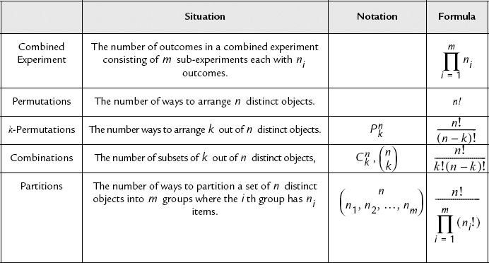
Naturally, there are many more formulas of this nature for more complicated scenarios. We make no attempt to give any sort of exhaustive coverage here. Rather, we merely include some of the more commonly encountered situations in the field of combinatorics. Table 2.2 summarizes the results we have developed and provides a convenient place to find relevant formulas for future reference. In that table, we have also included the notation pnk to represent the number of k-permutations of n items and cnk to represent the number of combinations of k out of n items. This notation, or some variation of it, is commonly used in many textbooks as well as in many popularly used calculators.
Table 2.2. Summary of combinatorics formulas
2.6 Bayes’s Theorem
In this section, we develop a few results related to the concept of conditional probability. While these results are fairly simple, they are so useful that we felt it was appropriate to devote an entire section to them. To start with, the following theorem was essentially proved in the previous section and is a direct result of the definition of conditional probability.
Theorem 2.9: For any events A and B such that Pr(B) ≠ 0,
![]() (2.19)
(2.19)
Proof: From Definition 2.5,
![]() (2.20)
(2.20)
Theorem 2.9 follows directly by dividing the preceding equations by Pr(B).
Theorem 2.9 is useful for calculating certain conditional probabilities since, in many problems, it may be quite difficult to compute Pr(A|B) directly, whereas calculating Pr(B|A) may be straightforward.
Theorem 2.10 (Theorem of Total Probability): Let B1, B2, …, Bn be a set of mutually exclusive and exhaustive events. That is, Bi ∩ Bj = Ø for all i ≠ j and
 (2.21)
Then
 (2.22)
Proof: As with Theorem 2.1, a Venn diagram (shown in Figure 2.2) is used here to aid in the visualization of our result. From the diagram, it can be seen that the event A can be written as

Figure 2.2 Venn diagram used to help prove the Theorem of Total Probability.
![]() (2.23)
(2.23)
![]() (2.24)
(2.24)
Also, since the Bi are all mutually exclusive, then the {A ∩ Bi } are also mutually exclusive so that
 (2.25)
 (2.26)
Finally by combining the results of Theorems 2.9 and 2.10, we get what has come to be know as Bayes’s theorem.
Theorem 2.11 (Bayes’s Theorem): Let B1, B2, …, Bn be a set of mutually exclusive and exhaustive events. Then,
 (2.27)
As a matter of nomenclature, Pr(Bi ) is often referred to as the a priori1 probability of event Bi, while Pr(Bi|A) is known as the a posteriori2 probability of event Bi given A. Section 2.9 presents an engineering application showing how Bayes’s theorem is used in the field of signal detection. We conclude here with an example showing how useful Bayes’s theorem can be.
Example 2.20
A certain auditorium has 30 rows of seats. Row 1 has 11 seats, while Row 2 has 12 seats, Row 3 has 13 seats, and so on to the back of the auditorium where Row 30 has 40 seats. A door prize is to be given away by randomly selecting a row (with equal probability of selecting any of the 30 rows) and then randomly selecting a seat within that row (with each seat in the row equally likely to be selected). Find the probability that Seat 15 was selected given that Row 20 was selected and also find the probability that Row 20 was selected given that Seat 15 was selected. The first task is straightforward. Given that Row 20 was selected, there are 30 possible seats in Row 20 that are equally likely to be selected. Hence, Pr(Seat 15|Row 20) = 1/30. Without the help of Bayes’s Theorem, finding the probability that Row 20 was selected given that we know Seat 15 was selected would seem to be a formidable problem. Using Bayes’s Theorem,
Pr(Row 20|Seat 15) = Pr(Seat 15|Row 20)Pr(Row 20)/Pr(Seat 15).
The two terms in the numerator on the right hand side are both equal to 1/30. The term in the denominator is calculated using the help of the theorem of total probability.
![]()
With this calculation completed, the a posteriori probability of Row 20 being selected given seat 15 was selected is given by

Note that the a priori probability that Row 20 was selected is 1/30 = 0.0333. Therefore, the additional information that Seat 15 was selected makes the event that Row 20 was selected slightly less likely. In some sense, this may be counterintuitive, since we know that if Seat 15 was selected, there are certain rows that could not have been selected (i.e., Rows 1-4 have less that 15 seats) and, therefore, we might expect Row 20 to have a slightly higher probability of being selected compared to when we have no information about what seat was selected. To see why the probability actually goes down, try computing the probability that Row 5 was selected given the Seat 15 was selected. The event that Seat 15 was selected makes some rows much more probable while it makes others less probable and a few rows now impossible.
2.7 Independence
In Example 2.20, it was seen that observing one event can change the probability of the occurrence of another event. In that particular case, the fact that it was known that Seat 15 was selected lowered the probability that Row 20 was selected. We say that the event A = {Row 20 was selected} is statistically dependent on the event B = {Seat 15 was selected}. If the description of the auditorium were changed so that each row had an equal number of seats (e.g., say all 30 rows had 20 seats each), then observing the event B={Seat 15 was selected} would not give us any new information about the likelihood of the event A = {Row 20 was selected}. In that case, we say that the events A and B are statistically independent. Mathematically, two events A and B are independent if Pr(A|B) = Pr(A). That is, the a priori probability of event A is identical to the a posteriori probability of A given. Note that if Pr(A|B) = Pr(A), then the following two conditions also hold (see Exercise 2.22)
![]() (2.28)
(2.28)
![]() (2.29)
(2.29)
Furthermore, if Pr(A|B) ≠ Pr(A), then the other two conditions also do not hold. We can thereby conclude that any of these three conditions can be used as a test for independence and the other two forms must follow. We use the last form as a definition of independence since it is symmetric relative to the events A and B.
Definition 2.6: Two events are statistically independent if and only if
![]() (2.30)
(2.30)
Example 2.21
Consider the experiment of tossing two numbered dice and observing the numbers that appear on the two upper faces. For convenience, let the dice be distinguished by color, with the first die tossed being red and the second being white. Let A = {number on the red die is less than or equal to 2}, B = {number on the white die is greater than or equal to 4}, and C = {the sum of the numbers on the two dice is 3}. As mentioned in the preceding text, there are several ways to establish independence (or lack thereof) of a pair of events. One possible way is to compare Pr(A, B) with Pr(A)Pr(B). Note that for the events defined here, Pr(A) = 1/3, Pr(B) = 1/2, and Pr(C) = 1/18. Also, of the 36 possible atomic outcomes of the experiment, 6 belong to the event A ∩ B and hence Pr(A, B) = 1/6. Since Pr(A)Pr(B) = 1/6 as well, we conclude that the events A and B are independent. This agrees with intuition since we would not expect the outcome of the roll of one die to effect the outcome of the other. What about the events A and C? Of the 36 possible atomic outcomes of the experiment, two belong to the event A ∩ C and hence Pr(A, C) = 1/18. Since Pr(A)Pr(C) = 1/54, the events A and C are not independent. Again, this is intuitive since whenever the event C occurs, the event A must also occur and so these two must be dependent. Finally, we look at the pair of events B and C. Clearly, B and C are mutually exclusive. If the white die shows a number greater than or equal to 4, there is no way the sum can be 3. Hence Pr(B, C) = 0, and since Pr(B)Pr(C) = 1/36, these two events are also dependent.
The previous example brings out a point that is worth repeating. It is a common mistake to equate mutual exclusiveness with independence. Mutually exclusive events are not the same thing as independent events. In fact, for two events A and B for which Pr(A) ≠ 0 and Pr(B) ≠ 0, A and B can never be both independent and mutually exclusive. Thus, mutually exclusive events are necessarily statistically dependent.
A few generalizations of this basic idea of independence are in order. First, what does it mean for a set of three events to be independent? The following definition clarifies this and then we generalize the definition to any number of events.
Definition 2.7: The events A, B, and C are mutually independent if each pair of events is independent; that is
![]() (2.31a)
(2.31a)
![]() (2.31b)
(2.31b)
![]() (2.31c)
(2.31c)
and in addition,
![]() (2.31d)
(2.31d)
Definition 2.8: The events A1, A2, …, An are independent if any subset of k ≤ n of these events are independent, and in addition
![]() (2.32)
(2.32)
There are basically two ways in which we can use this idea of independence. As was shown in Example 2.21, we can compute joint or conditional probabilities and apply one of the definitions as a test for independence. Alternatively, we can assume independence and use the definitions to compute joint or conditional probabilities that otherwise may be difficult to find. This latter approach is used extensively in engineering applications. For example, certain types of noise signals can be modeled in this way. Suppose we have some time waveform X(t) which represents a noisy signal which we wish to sample at various points in time, t1, t2, …, tn . Perhaps, we are interested in the probabilities that these samples might exceed some threshold, so we define the events Ai = Pr(X(ti ) > T), i = 1, 2, …, n. How might we calculate the joint probability Pr(A1, A2, …, An )? In some cases, we have every reason to believe that the value of the noise at one point in time does not effect the value of the noise at another point in time. Hence, we assume that these events are independent and write Pr(A1, A2, …, An ) = Pr(A1)Pr(A2) … Pr(An ).
Example 2.22
Consider a communications network with nodes A, B, C, and D and links a1, a2, a3, and a4, as shown in the diagram. The probability of a link being available at any time is p. In order to send a messsage from node A to node D we must have a path of available links from A to D. Assuming independence of link availability, what is the probability of being able to send a message? Let Lk be the event that link ak is available. Then

2.8 Discrete Random Variables
Suppose we conduct an experiment, E, which has some sample space, S. Furthermore, let ξ; be some outcome defined on the sample space, S. It is useful to define functions of the outcome ξ;, X = f(ξ;). That is, the function f has as its domain all possible outcomes associated with the experiment, E. The range of the function f will depend upon how it maps outcomes to numerical values but in general will be the set of real numbers or some part of the set of real numbers. Formally, we have the following definition.
Definition 2.9: A random variable is a real valued function of the elements of a sample space, S. Given an experiment, E, with sample space, S, the random variable X maps each possible outcome, ξ; ∈ S, to a real number X(ξ;) as specified by some rule. If the mapping X(ξ;) is such that the random variable X takes on a finite or countably infinite number of values, then we refer to X as a discrete random variable; whereas, if the range of X(ξ;) is an uncountably infinite number of points, we refer to X as a continuous random variable.
Since X = f(ξ;) is a random variable whose numerical value depends on the outcome of an experiment, we cannot describe the random variable by stating its value; rather, we must give it a probabilistic description by stating the probabilities that the variable X takes on a specific value or values (e.g., Pr(X=3) or Pr(X > 8)). For now, we will focus on random variables which take on discrete values and will describe these random variables in terms of probabilities of the form Pr(X=x). In the next chapter when we study continuous random variables, we will find this description to be insufficient and will introduce other probabilistic descriptions as well.
Definition 2.10: The probability mass function (PMF), PX (x), of a random variable, X, is a function that assigns a probability to each possible value of the random variable, X. The probability that the random variable X takes on the specific value x is the value of the probability mass function for x. That is, PX (x) = Pr(X=x). We use the convention that upper case variables represent random variables while lower case variables represent fixed values that the random variable can assume.
Example 2.23
A discrete random variable may be defined for the random experiment of flipping a coin. The sample space of outcomes is S = {H, T}. We could define the random variable X to be X(H) = 0 and X(T) = 1. That is, the sample space H, T is mapped to the set {0, 1} by the random variable X. Assuming a fair coin, the resulting probability mass function is PX (0) = 1/2 and PX (l) = 1/2. Note that the mapping is not unique and we could have just as easily mapped the sample space {H, T} to any other pair of real numbers (e.g., {1,2}).
Example 2.24
Suppose we repeat the experiment of flipping a fair coin n times and observe the sequence of heads and tails. A random variable, Y, could be defined to be the number of times tails occurs in n trials. It turns out that the probability mass function for this random variable is
![]()
The details of how this PMF is obtained will be deferred until later in this section.
Example 2.25
Again, let the experiment be the flipping of a coin, and this time we will continue repeating the event until the first time a heads occurs. The random variable Z will represent the number of times until the first occurrence of a heads. In this case, the random variable Z can take on any positive integer value, 1 ≤ Z ≤ ∞. The probability mass function of the random variable Z can be worked out as follows:
![]()
Hence,
PZ (n) = 2−n, n = 1, 2, 3,….
Example 2.26
In this example, we will estimate the PMF in Example 2.24 via MATLAB simulation using the relative frequency approach. Suppose the experiment consists of tossing the coin n = 10 times and counting the number of tails. We then repeat this experiment a large number of times and count the relative frequency of each number of tails to estimate the PMF. The following MATLAB code can be used to accomplish this. Results of running this code are shown in Figure 2.3.

Figure 2.3 MATLAB Simulation results from Example 2.26.

Try running this code using a larger value for m. You should see more accurate relative frequency estimates as you increase m.
From the preceding examples, it should be clear that the probability mass function associated with a random variable, X, must obey certain properties. First, since PX (x) is a probability it must be non-negative and no greater than 1. Second, if we sum PX (x) over all x, then this is the same as the sum of the probabilities of all outcomes in the sample space, which must be equal to 1. Stated mathematically, we may conclude that
![]() (2.33a)
(2.33a)
![]() (2.33b)
(2.33b)
When developing the probability mass function for a random variable, it is useful to check that the PMF satisfies these properties.
In the paragraphs that follow, we list some commonly used discrete random variables, along with their probability mass functions, and some real-world applications in which each might typically be used.
A. Bernoulli Random Variable
This is the simplest possible random variable and is used to represent experiments which have two possible outcomes. These experiments are called Bernoulli trials and the resulting random variable is called a Bernoulli random variable. It is most common to associate the values {0,1} with the two outcomes of the experiment. If X is a Bernoulli random variable, its probability mass function is of the form
![]() (2.34)
(2.34)
The coin tossing experiment would produce a Bernoulli random variable. In that case, we may map the outcome H to the value X = 1 and T to X = 0. Also, we would use the value p = 1/2 assuming that the coin is fair. Examples of engineering applications might include radar systems where the random variable could indicate the presence (X = 1) or absence (X = 0) of a target, or a digital communication system where X = 1 might indicate a bit was transmitted in error while X = 0 would indicate that the bit was received correctly. In these examples, we would probably expect that the value of p would be much smaller than 1/2.
B. Binomial Random Variable
Consider repeating a Bernoulli trial n times, where the outcome of each trial is independent of all others. The Bernoulli trial has a sample space of S = {0,1} and we say that the repeated experiment has a sample space of Sn = { 0, 1 }n, which is referred to as a Cartesian space. That is, outcomes of the repeated trials are represented as n element vectors whose elements are taken from S. Consider, for example, the outcome
![]()
(2.35)
The probability of this outcome occurring is
 (2.36)
In fact, the order of the 1’s and 0’s in the sequence is irrelevant. Any outcome with exactly k 1’s and n − k 0’s would have the same probability. Now let the random variable X represent the number of times the outcome 1 occurred in the sequence of n trials. This is known as a binomial random variable and takes on integer values from 0 to n. To find the probability mass function of the binomial random variable, let Ak be the set of all outcomes which have exactly k 1’s and n − k 0’s. Note that all outcomes in this event occur with the same probability. Furthermore, all outcomes in this event are mutually exclusive. Then,
PX (k) = Pr(Ak ) = (# of outcomes in Ak )*(probability of each outcome in Ak
 (2.37)
The number of outcomes in the event Ak is just the number of combinations of n objects taken k at a time. Referring to Theorem 2.7, this is the binomial coefficient,
![]() (2.38)
(2.38)
As a check, we verify that this probability mass function is properly normalized:
 (2.39)
In the above calculation, we have used the binomial expansion
 (2.40)
Binomial random variables occur, in practice, any time Bernoulli trials are repeated. For example, in a digital communication system, a packet of n bits may be transmitted and we might be interested in the number of bits in the packet that are received in error. Or, perhaps a bank manager might be interested in the number of tellers that are serving customers at a given point in time. Similarly, a medical technician might want to know how many cells from a blood sample are white and how many are red. In Example 2.23, the coin tossing experiment was repeated n times and the random variable Y represented the number of times tails occurred in the sequence of n tosses. This is a repetition of a Bernoulli trial, and hence the random variable Y should be a binomial random variable with p = 1/2 (assuming the coin is fair).
C. Poisson Random Variable
Consider a binomial random variable, X, where the number of repeated trials, n, is very large. In that case, evaluating the binomial coefficients can pose numerical problems. If the probability of success in each individual trial, p, is very small, then the binomial random variable can be well approximated by a Poisson random variable. That is, the Poisson random variable is a limiting case of the binomial random variable. Formally, let n approach infinity and p approach 0 in such a way that ![]() . Then, the binomial probability mass function converges to the form
. Then, the binomial probability mass function converges to the form
![]() (2.41)
(2.41)
which is the probability mass function of a Poisson random variable. We see that the Poisson random variable is properly normalized by noting that
![]() (2.42)
(2.42)
(see Equation E.14 in Appendix E). The Poisson random variable is extremely important as it describes the behavior of many physical phenomena. It is commonly used in queuing theory and in communication networks. The number of customers arriving at a cashier in a store during some time interval may be well modeled as a Poisson random variable as may the number of data packets arriving at a node in a computer network. We will see increasingly in later chapters that the Poisson random variable plays a fundamental role in our development of a probabilistic description of noise.
D. Geometric Random Variable
Consider repeating a Bernoulli trial until the first occurrence of the outcome ξ;0. If X represents the number of times the outcome ξ;1 occurs before the first occurrence of ξ;0, then X is a geometric random variable whose probability mass function is
![]() (2.43)
(2.43)
We might also formulate the geometric random variable in a slightly different way. Suppose X counted the number of trials that were performed until the first occurrence of ξ;0. Then, the probability mass function would take on the form,
![]() (2.44)
(2.44)
The geometric random variable can also be generalized to the case where the outcome ξ;0 must occur exactly m times. That is, the generalized geometric random variable counts the number of Bernoulli trials that must be repeated until the mth occurrence of the outcome ξ;0. We can derive the form of the probability mass function for the generalized geometric random variable from what we know about binomial random variables. For the mth occurrence of ξ;0 to occur on the £th trial, the first k−1 trials must have had m−1 occurrences of ξ;0 and k−m occurrences of ξ;1. Then
Px (k) = Pr({((m − 1) occurrences of ξ;0 in k − 1) trials } ∩ {ξ;0 occurs on the kth trial}
![]() (2.45)
(2.45)
This generalized geometric random variable sometimes goes by the name of a Pascal random variable or the negative binomial random variable.
Of course, one can define many other random variables and develop the associated probability mass functions. We have chosen to introduce some of the more important discrete random variables here. In the next chapter, we will introduce some continuous random variables and the appropriate probabilistic descriptions of these random variables. However, to close out this chapter, we provide a section showing how some of the material covered herein can be used in at least one engineering application.
2.9 Engineering Application—An Optical Communication System
Figure 2.4 shows a simplified block diagram of an optical communication system. Binary data are transmitted by pulsing a laser or a light emitting diode (LED) that is coupled to an optical fiber. To transmit a binary 1, we turn on the light source for T seconds, while a binary 0 is represented by turning the source off for the same time period. Hence, the signal transmitted down the optical fiber is a series of pulses (or absence of pulses) of duration T seconds which represents the string of binary data to be transmitted. The receiver must convert this optical signal back into a string of binary numbers; it does this using a photodetector. The received light wave strikes a photoemissive surface, which emits electrons in a random manner. While the number of electrons emitted during a T second interval is random and thus needs to be described by a random variable, the probability mass function of that random variable changes according to the intensity of the light incident on the photoemissive surface during the T second interval. Therefore, we define a random variable X to be the number of electrons counted during a T second interval, and we describe this random variable in terms of two conditional probability mass functions, PX| 0(k) = Pr(X =k|0 sent) and P X|1(k) = Pr(X =k|1 sent). It can be shown through a quantum mechanical argument that these two probability mass functions should be those of Poisson random variables. When a binary 0 is sent, a relatively low number of electrons are typically observed; whereas, when a 1 is sent, a higher number of electrons is typically counted. In particular, suppose the two probability mass functions are given by

Figure 2.4 Block diagram of an optical communication system.
![]() (2.46a)
(2.46a)
![]() (2.46b)
(2.46b)
In these two PMFs, the parameters R0 and R1 are interpreted as the “average” number of electrons observed when a 0 is sent and when a 1 is sent, respectively. Also, it is assumed that R0 ≤ R1, so when a 0 is sent we tend to observe fewer electrons than when a 1 is sent.
At the receiver, we count the number of electrons emitted during each T second interval and then must decide whether a “0” or “1” was sent during each interval. Suppose that during a certain bit interval it is observed that k electrons are emitted. A logical decision rule would be to calculate Pr(0 sent X =k) and Pr(1 sent X =k) and choose according to whichever is larger. That is, we calculate the a posteriori probabilities of each bit being sent, given the observation of the number of electrons emitted and choose the data bit which maximizes the a posteriori probability. This is referred to as a maximum a posteriori (MAP) decision rule and we decide that a binary 1 was sent if
![]() (2.47)
(2.47)
otherwise, we decide a 0 was sent. Note that these desired a posteriori probabilities are backward relative to how the photodetector was statistically described. That is, we know the probabilities of the form Pr(X =k 1 sent) but we want to know Pr(1 sent X =k). We call upon Bayes’s theorem to help us convert what we know into what we desire to know. Using the theorem of total probability,
![]() (2.48)
(2.48)
The a priori probabilities Pr(0 sent) and Pr(1 sent) are taken to be equal (to 1/2), so that
![]() (2.49)
(2.49)
Therefore, applying Bayes’s theorem,
 (2.50)
and
 (2.51)
Since the denominators of both a posteriori probabilities are the same, we decide that a 1 was sent if
![]() (2.52)
(2.52)
After a little algebraic manipulation, this reduces down to choosing in favor of a 1 if
 (2.53)
otherwise, we choose in favor of 0. That is, the receiver for our optical communication system counts the number of electrons emitted and compares that number with a threshold. If the number of electrons emitted is above the threshold, we decide that a 1 was sent; otherwise, we decide a 0 was sent.
We might also be interested in evaluating how often our receiver makes a wrong decision. Ideally, the answer is that errors are very rare, but still we would like to quantify this. Toward that end, we note that errors can occur in two manners. First a 0 could be sent and the number of electrons observed could fall above the threshold, causing us to decide that a 1 was sent. Likewise, if a 1 is actually sent and the number of electrons observed is low, we would mistakenly decide that a 0 was sent. Again, invoking concepts of conditional probability, we see that
![]() (2.54)
(2.54)
Let x0 be the threshold with which we compare X to decide which data bit was sent. Specifically, let3![]() so that we decide a 1 was sent if X > x0, and we decide a 0 was sent if X ≤ x0. Then
so that we decide a 1 was sent if X > x0, and we decide a 0 was sent if X ≤ x0. Then
 (2.55)
Likewise,
 (2.56)
Hence, the probability of error for our optical communication system is
 (2.57)
Figure 2.5 shows a plot of the probability of error as a function of R1 with R0 as a parameter. The parameter R0 is a characteristic of the photodetector used. We will see in later chapters that R0 can be interpreted as the “average” number of electrons emitted during a bit interval when there is no signal incident on the photodetector. This is sometimes referred to as the “dark current.” The parameter R1 is controlled by the intensity of the incident light. Given a certain photodetector, the value of the parameter R0 can be measured. The required value of R1 needed to achieve a desired probability of error can be found from Figure 2.5 (or from Equation 2.57 which generated that figure). The intensity of the laser or LED can then be adjusted to produce the required value for the parameter R1.

Figure 2.5 Probability of error curves for an optical communication system; curves are parameterized from bottom to top with R0 =1, 2, 4, 7, 10.
Exercises
Section 2.1: Experiments, Sample Spaces, and Events
2.1 An experiment consists of rolling n (six-sided) dice and recording the sum of the n rolls. How many outcomes are there to this experiment?
(a) An experiment consists of rolling a die and flipping a coin. If the coin flip is heads, the value of the die is multiplied by –1, otherwise it is left as is. What are the possible outcomes of this experiment?
(b) Now, suppose we want to repeat the experiment in part (a) n times and record the sum of the results of each experiment. How many outcomes are there in this experiment and what are they?
2.3 An experiment consists of selecting a number x from the interval [0, 1) and a number y from the interval [0, 2) to form a point (x, y).
(a) Describe the sample space of all points.
(b) What fraction of the points in the space satisfy x > y?
(c) What fraction of points in the sample space satisfy x = y?
2.4 An experiment consists of selecting a point (x, y) from the interior of the unit circle, x2 + y2 ≤ 1.
(a) What fraction of the points in the space satisfy ![]() ?
?
(b) What fraction of the points in the space satisfy ![]() ?
?
2.5 An experiment consists of selecting two integers (n, k) such that 0 ≤ n ≤ 5 and 0 ≤ k ≤ 10.
(a) How many outcomes are in the sample space?
(b) What fraction of the outcomes in the sample space satisfy n > k?
(c) What fraction of the outcomes in the sample space satisfy n ≤ k?
(d) What fraction of the outcomes in the sample space satisfy n = k?
(a) For each of the experiments described in Examples 2.1-2.5, state whether or not it is reasonable to expect that each outcome of the experiment would occur equally often.
(b) Create (a hypothethical) experiment of your own with a finite number of outcomes where you would not expect the outcomes to occur equally often.
Section 2.2 Axioms of Probability
2.7 Using mathematical induction, prove Corollary 2.1. Recall, Corollary 2.1 states that for M events A1, A2, …, AM
which are mutually exclusive (i.e., Ai
∩ Aj
= Ø for all i ≠ j),

2.8 Develop a careful proof of Theorem 2.1 which states that for any events A and B,
![]()
One way to approach this proof is to start by showing that the set A ∪ B can be written as the union of three mutually exclusive sets,
![]()
and hence by Corollary 2.1,
![]()
![]()
![]()
(Hint: recall DeMorgan’s law) Put these results together to complete the desired proof.
2.9 Show that the above formula for the probability of the union of two events can be generalized to three events as follows:

2.10 Prove Theorem 2.3 which states that if A ⊂ B then Pr(A) ≤ Pr(B).
2.11 Formally prove the union bound which states that for any events A1, A2, …, AM
(not necessarily mutually exclusive),

2.12 An experiment consists of tossing a coin twice and observing the sequence of coin tosses. The sample space consists of four outcomes ξ;1 = (H, H), ξ;2 = (H, T), ξ;3 = (T, H), and ξ;4 = (T, T). Suppose the coin is not evenly weighted such that we expect a heads to occur more often than tails and as a result, we assign the following probabilities to each of the four outcomes:
![]()
(a) Does this probability assignment satisfy the three axioms of probability?
(b) Given this probability assignment, what is Pr(first toss is heads)?
(c) Given this probability assignment, what is Pr(second toss is heads)?
2.13 Repeat Exercise 2.12 if the probability assignment is changed to:
![]()
2.14 Consider the experiment of tossing a six-sided die as described in Example 2.2. Suppose the die is loaded and as such we assign the following probabilities to each of the six outcomes:
![]()
Is this assignment consistent with the three axioms of probability?
Section 2.3 Assigning Probabilities
2.15 Demonstrate that the relative frequency approach to assigning probabilities satisfies the three axioms of probability.
2.16 We are given a number of darts. Suppose it is known that each time we throw a dart at a target, we have a probability of 1/4 of hitting the target. An experiment consists of throwing three darts at the target and observing the sequence of hits and misses (e.g., one possible outcome might be (H, M, M)).
(a) Find a probabilty assignment for the eight outcomes of this experiment that leads to a probabilty of 1/4 of hitting the target on any toss. Note, your assignment must satisfy the axioms of probability.
(b) Is the probability assigment you chose unique? That is, are there other possible probability assignments that lead to a probabilty of 1/4 of hitting the target on any toss, or is yours the only valid assignment? Carefully prove your answer.
2.17 A spinner as shown in the figure selects a number from the set {1, 2, 3, 4}. If we select the outcomes {ξ;1 = 1, ξ;2 = 2, ξ;3 = 3, ξ;4 = 4} as atomic outcomes and use the classical approach to assigning probabilities, then we would conclude that the spinner selects all four numbers each with equal probability, 1/4. Show how to describe this experiment in terms of more fundamental outcomes so that the classical approach leads to a more reasonable probability assignment.

2.18 Consider a modified version of the experiment in Example 2.4 where we flip a coin until the first occurence of tails or until we flip the coin four times, whichever comes first.
(a) List the possible outcomes of this experiment. How many are there? Would you expect each outcome to be equally probable?
(b) Can you develop a method to use the classical approach to assign probabilities to this experiment? Hint: You are going to have to define an atomic outcome which is more fundamental than the outcomes listed in part (a).
(c) Given the probability assigment you developed in part (b), find the probabilities of each outcome listed in part (a).
2.19 Extend your solution to Exercise 2.18 to find the probability of each of the outcomes of Example 2.4.
2.20 If we roll two dice and observe the sum, the most common outcome is 7 and occurs with probability 1/6. But what if we roll more than 2 dice?
Section 2.4 Joint and Conditional Probabilities
2.21 Demonstrate that the definition of conditional probability Pr(A|B) = Pr(A, B)Pr(B) satisfies the three axioms of probability.
2.22 Prove that if Pr(B|A) = Pr(B), then it follows that
(b) Pr(A|B) = Pr(A).
Furthermore, show that if Pr(B|A) ≠ Pr(B), then the two conditions above do not hold as well.
2.23 A box of 30 diodes is known to contain five defective ones. If two diodes are selected at random without replacement, what is the probability that at least one of these diodes is defective?
2.24 Two balls are selected sequentially (without replacement) from an urn containing three red, four white, and five blue balls.
(a) What is the probability that the first is red and the second blue?
(b) What is the probability of selecting a white ball on the second draw if the first ball is replaced before the second is selected?
(c) What is the probability of selecting a white ball on the second draw if the first ball is not replaced before the second is selected?
2.25 Two six-sided (balanced) dice are thrown. Find the probabilities of each of the following events:
(a) a 5 does not occur on either throw;
(c) a 5 and a 3 occur in any order;
(d) the first throw is a 5 and the second throw is a 5 or a 4;
2.26 Two six-sided (balanced) dice are thrown. Find the probabilities of each of the following events:
(a) only 2, 3, or 4 appear on both dice;
(b) the value of the second roll subtracted from the value of the first roll is 2;
(c) the sum is 10 given that one roll is 6;
2.27 Consider two events A and B such that Pr(A) > Pr(B). Determine if Fr(A|B) ≥ Pr(B|A) is always true, sometimes true, or never true.
2.28 Prove that for any two events A and B, Pr(A ∩ B) ≤ Pr(A) ≤ Pr(A ∪ B).
Section 2.5: Basic Combinatorics
2.29 Use mathematical induction to prove Theorem 2.4. Recall that Theorem 2.4 states that a combined experiment, E = E1 × E2 × E3 × … ×Em, consisting of experiments Ei
each with ni
outcomes, i = 1, 2, 3, …, m, has a total number of possible outcomes given by
![]()
2.30 Use mathematical induction to prove Theorem 2.8. Recall that Theorem 2.8 states that given a set of n distinct elements, the number of ways to partition the set into m groups where the ith group has ni
elements is given by the multinomial coefficient,
![]()
2.31 Prove the following identities involving the binomial coefficient ![]() .
.
2.32 I deal myself 3 cards from a standard 52-card deck. Find the probabilities of each of the following events:
(a) 2 of a kind (e.g., 2 fives or 2 kings);
(c) 3 of the same suit (a.k.a a flush, e.g., 3 hearts or 3 clubs);
(d) 3 cards in consecutive order (a.k.a. a straight, e.g., 2-3-4 or 10-J-Q).
2.33 I deal myself 13 cards for a standard 52-card deck. Find the probabilities of each of the following events:
(a) exactly one heart appears in my hand (of 13 cards);
2.34 For an alphabet consisting of 26 characters, find the following:
(a) The number of possible 4-letter sequences (words) where the same letter can appear in the word more than once.
(b) The number of possible 4-letter sequences (words) where the same letter cannot appear in the word more than once.
(c) The number of different ways the 26 letters can be ordered.
2.35 In pulse-code modulation (PCM), a PCM word consists of a sequence of binary digits (bits) of 1s and 0s.
(a) Suppose the PCM word length is n bits long. How many distinct words are there?
(b) If each PCM word, three bits long, is equally likely to occur, what is the probability of a word with exactly two 1s to occur?
2.36 In pulse-amplitude modulation (PAM), a PAM word consists of a sequence of pulses, where each pulse may take on a given number of amplitude levels. Suppose a PAM word is n pulses long and each pulse may take on m different levels.
(a) How many distinct PAM words are there?
(b) If each PAM word, 4 pulses long, is equally likely to occur and each pulse can have one of three levels, {0, 1, 2}, what is the probability of a PAM word occurring with exactly two pulses of level 2?
2.37 A certain communication system transmits text messages by representing each character with an n-bit binary codeword. Suppose it is necessary for this communication system to operate in such a way that there are always an equal number of 0s and 1s transmitted. Toward that end, the communication system uses a codebook consisting only of those n-bit words that have exactly n/2 0s and n/2 1s (where n is an even integer). For example, in the case of n = 4, there are exactly 6 four-bit codewords consisting of exactly two 1s and two 0s resulting in the codebook {(1100), (1010), (1001), (0110), (0101), (0011)}. Thus, with four bit codewords, we could represent an alphabet of only six characters.
(a) Find an expression for the number of codewords with half 1s and half 0s for an arbitrary even integer n.
(b) What is the minimum length of codeword we would need if the codebook needs to represent at least 100 different characters?
2.38 Phone numbers in the United States consist of 10 digits, a three-digit area code followed by a seven-digit number. Suppose there are several constraints that must be satisfied for a phone number to be valid, such as:
(i) Neither the first digit of any area code nor the first digit of a phone number can be 0, (since 0 is reserved to connenct to an operator).
(ii) The second digit of any valid area code must be either 0 or 1.
(iii) The second digit of any valid phone number must not be either 0 or 1 (the second and third constraints are no longer in place but were once used so that the phone company could easily determine whether you were making a local or long distance call).
(iv) The second and third digits of any valid area code cannot both be 1s.
(v) The second and third digits of any valid phone number cannot both be 1s. (three-digit numbers ending in 11 are reserved for special purposes, e.g., emergency, 911, or information, 411).
(a) Given the five constraints listed above, how many valid three-digit area codes are there?
(b) Given the five constraints listed above, how many valid seven-digit phone numbers are there?
(c) How many different 10-digit phone numbers can be constructed under these constraints?
2.39 A balanced coin is tossed nine times. Find the probabilities of each of the following events:
2.40 A blackjack hand consists of 2 cards drawn from a 52-card deck. The order in which the cards are drawn does not matter.
(a) How many different blackjack hands are there?
(b) In blackjack, the suit of the card is irrelevant to the game. If we do not make a distinction between the different suits, now how many different blackjack hands are there?
(c) In blackjack, 10s, Jacks, Queens, and Kings are all worth 10 points and thus have an identical function in the game. If we do not make a distinction between 10s, Jacks, Queens, and Kings, nor between the different suits, now how many blackjack hands are there?
2.41 In the game of blackjack, Aces are worth 11 points (or they can also be counted as 1 point, but for the sake of this problem, we will only count them as 11 points), 10s, Jacks, Queens, and Kings are all worth 10 points and the other numbered cards are worth their face values (i.e., 2s are worth two points, 3s are worth three points, etc.). The suit of the card does not matter.
(a) Find the probability of being dealt a two-card blackjack hand worth a total of 18 or more points?
(b) Find the probability of being dealt a two-card blackjack hand worth a total of no less than 12 points and no more than 17 points?
Hint: Consider carefully the results of Problem 2.40 and think about what consists of an atomic outcome in this experiment.
2.42 In a game of blackjack, the player and the dealer are both dealt two cards. One of the dealer’s cards is dealt face up so that the player gets to see it. Suppose you (as a player) are dealt a 10 and a 6 and you observe that one of the dealer’s cards is a 7. Given the three observed cards, what is the probability that the dealers cards total more points than yours (before any additional cards are drawn)? Refer to Exercise 2.41 for a description of the point values of various cards in blackjack.
2.43 A poker hand consists of 5 cards drawn from a 52-card deck.
(a) How many different poker hands are there?
(b) How many different poker hands are there that contain all four aces? What then is the probability of being dealt four aces? What is the probability of being dealt four of a kind (i.e., four aces, or four kings, or four queens, etc.)?
(c) How many different poker hands are there that contain exactly three aces? What then is the probability of being dealt three aces? What is the probability of being dealt three of a kind (i.e., three aces, or three kings, or three queens, etc.)?
2.44 A certain gym teacher has a class of 20 students. He wants to divide them into four teams of five students each in order to have a class basketball tournament.
(a) How many different ways can he divide the class into four teams?
(b) Tommy and Bobby are two of the students in the class and are best friends. Assuming the gym teacher assigns students in a completely random fashion, what is the probability that they get selected to be on the same team?
(c) Neither boy wants to be on a team with the class bully, Frank. What is the probability that neither Tommy nor Bobby are on the same team as Frank?
Section 2.6: Bayes’s Theorem
2.45 Manufacturer X produces personal computers (PCs) at two different locations in the world. Fifteen percent of the PCs produced at location A are delivered to a retail outlet defective, while five percent of the PCs produced at location B are delivered defective to the same retail store. If the manufacturing plant at A produces 1,000,000 PCs per year and the plant at B produces 150,000 PCs per year, find the probability of purchasing a defective PC.
2.46 A communication system sends binary data {0 or 1} which is then detected at the receiver. The receiver occasionally makes mistakes and sometimes a 0 is sent and is detected as a 1 or a 1 can be sent and detected as a 0. Suppose the communication system is described by the following set of conditional probabilities:
Pr(0 received|0 transmitted) = 0.95, Pr(1 received|0 transmitted) = 0.05
Pr(0 received)|1 transmitted) = 0.10, Pr(1 received)|1 transmitted) = 0.90
(a) Assuming 0s and 1s are equally likely to be transmitted (i.e.,
Pr(0 transmitted) = 1/2 and Pr(1 transmitted) = 1/2), find Pr(0 received) and Pr(1 received).
(b) Suppose a 0 is detected at the receiver. What is the probability that the transmitted bit was actually a 1? Also, if a 1 was detected at the receiver, what is the probability that the transmitted bit was actually a 0?
(c) What is the probability that the detected bit is not equal to the transmitted bit. This is the overall probability of error of the receiver.
2.47 In this problem, we will modify the communication system described in Exercise 2.46 so that the detector at the receiver is allowed to make one of three possible decisions:
| “0” | the detector decides the received signal was a 0, |
| “1” | the detector decides the received signal was a 1, |
| “E” | the detector is not sure and declares the received signal an erasure (i.e., the receiver chooses not to choose). |
The operation of the detector is described by the following set of conditional probabilities:
Pr(0 received | 0 transmitted) = 0.90, Pr(0 received 1 transmitted) = 0.04
Pr(1 received | 0 transmitted) = 0.01, Pr(1 received 1 transmitted) = 0.80
Pr(E received | 0 transmitted) = 0.09, Pr(E received 1 transmitted) = 0.16
Again, assume that 0s and 1s are equally likely to be transmitted.
(a) What is the probability that a symbol is erased at the receiver?
(b) Given that a received symbol is declared an erasure, what is the probability that a 0 was actually transmitted?
(c) What is the probability of error of this receiver? That is, what is the probability that a 0 was transmitted and it is detected as a 1 or a 1 was transmitted and it is detected as a 0?
2.48 We are in possession of two coins, one which is fairly balanced and turns up heads with probability 1/2, the other is weighted such that heads shows up with probability 3/4 and tails with probability 1/4. The two coins are identical looking and feeling so we cannot tell which is which. In order to determine which is the biased coin we toss the coin 10 times and observe the number of heads that occurred.
(a) If 7 heads were observed, what is the probability that the coin flipped was the fair coin?
(b) If 3 heads were observed, what is the probability that the coin flipped was the fair coin?
2.49 Researchers are investigating the physical development of children over time. In the study, children are given a physical aptitude test at several stages in their development. Let P be the event that the child passes the physical aptitude test. Furthermore, let B be the event that the child taking the test was a boy, and G be the event that the child taking the test was a girl. The computer storing the data from this project experienced hard drive failure and only some of the data was recovered resulting in the partial database shown in the table. Use your knowledge of probability theory to fill in the missing items in the table.
Data for Exercise 2.49

Section 2.7: Independence
2.50 Compare the two probability assignments in Exercises 2.12 and 2.13. Which of these two assignments corresponds to independent coin tosses?
2.51 Cards are drawn from a standard 52-card deck until an ace is drawn. After each card is drawn, it is put back in the deck and the cards are reshuffled so that each card drawn is independent of all others.
(a) Find the probability that the first ace is drawn on the 5th selection.
(b) Find the probability that at least 5 cards are drawn before the first ace appears.
(c) Repeat parts (a) and (b) if the cards are drawn without replacement. That is, after each card is drawn, the card is set aside and not replaced in the deck.
2.52 Cards are drawn from a standard 52-card deck until the third club is drawn. After each card is drawn, it is put back in the deck and the cards are reshuffled so that each card drawn is independent of all others.
(a) Find the probability that the 3rd club is drawn on the 8th selection.
(b) Find the probability that at least 8 cards are drawn before the 3rd club appears.
(c) Repeat parts (a) and (b) if the cards are drawn without replacement. That is, after each card is drawn, the card is set aside and not replaced in the deck.
2.53 A computer memory has the capability of storing 106 words. Due to outside forces, portions of the memory are often erased. Therefore, words are stored redundantly in various areas of the memory. If a particular word is stored in n different places in the memory, what is the probability that this word cannot be recalled if one-half of the memory is erased by electromagnetic radiation? Hint: Consider each word to be stored in a particular cell (or box).
These cells (boxes) may be located anywhere, geometrically speaking, in memory. The contents of each cell may be either erased or not erased. Assume n is small compared to the memory capacity.
2.54 If two events A and B are such that Pr(A) is not zero and Pr(B) is not zero, what combinations of independent (I), not independent (NI), mutually exclusive (M), and not mutually exclusive (NM) are permissible? In other words, which of the four combinations (I, M), (NI, M), (I, NM), and (NI, NM) are permissible? Construct an example for those combinations that are permissible.
2.55 Suppose two events A and B are independent.
(a) Is it true that A is independent of ![]() If yes, give a convincing proof, otherwise, give a counterexample.
If yes, give a convincing proof, otherwise, give a counterexample.
(b) Is it true that ![]() is independent of
is independent of ![]() If yes, give a convincing proof, otherwise, give a counterexample.
If yes, give a convincing proof, otherwise, give a counterexample.
2.56 Suppose we modify the communications network of Example 2.22 as shown in the diagram by adding a link from node B to node D. Assuming each link is available with probability p independent of any other link, what is the probability of being able to send a message from node A to D?
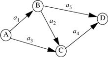
Section 2.8: Discrete Random Variables
2.57 A possible outcome of an experiment is the event A. The probability of this event is p. The experiment is performed n times, the outcome of any trial is not affected by the results of the previous trials. Define a random variable X to be the number of times the event A occurs in n trials.
2.58 For each of the following probability mass functions, find the value of the constant c:
(a) PX (k) = c(0.37)k, k = 0, 1, 2, …
(b) PX (k) = c(0.82)k, k = 1, 2, 3, …
(c) PX (k) = c(0.41)k, k = 0, 1, 2, …, 24.
2.59 Consider a Bernoulli trial where Pr(1) = p and Pr(0) = 1−p. Suppose this Bernoulli trial is repeated n times.
(a) Plot the probability mass function for a Binomial random variable, X, with p = 1/5 and n = 10.
(b) Plot the corresponding probability mass function for a Poisson random variable X with α = np = 2.
(c) Compare Pr(X ≥ 5) as computed by both the Binomial and Poisson random variables. Is the Poisson random variable a good approximation for the Binomial random variable for this example?
2.60 Suppose the arrival of telephone calls at a switch can be modeled with a Poisson PMF. That is, if X is the number of calls that arrive in t minutes, then
![]()
where λ is the average arrival rate in calls/minute. Suppose that the average rate of calls is 10 min.
(a) What is the probability that fewer than three calls will be received in the first 6 s?
(b) What is the probability that fewer than three calls will be received in the first 6 min?
2.61 In a certain lottery, six numbers are randomly chosen from the set {0, 1, 2, …, 49} (without replacement). To win the lottery, a player must guess correctly all six numbers but it is not necessary to specify in which order the numbers are selected.
(a) What is the probability of winning the lottery with only one ticket?
(b) Suppose in a given week, 6 million lottery tickets are sold. Suppose further that each player is equally likely to choose any of the possible number combinations and does so independent of the selections of all other players. What is the probability that exactly four players correctly select the winning combination?
(c) Again assuming 6 million tickets sold, what is the most probable number of winning tickets?
(d) Repeat parts (b) and (c) using the Poisson approximation to the binomial probability distribution. Is the Poisson distribution an accurate approximation in this example?
2.62 Imagine an audio amplifier contains six transistors. Harry has determined that two transistors are defective, but he does not know which two. Harry removes three transistors at random and inspects them. Let X be the number of defective transistors that Harry finds, where X may be 0, 1, or 2. Find the PMF for x.
2.63 A software manufacturer knows that l out of 10 software games that the company markets will be a financial success. The manufacturer selects 10 new games to market. What is the probability that exactly one game will be a financial success? What is the probability that at least two games will be a success?
2.64 In a digital communication system, a block of k data bits is mapped into an n-bit codeword that typically contains the k information bits as well as n − k redundant bits. This is known as an (n, k) block code. The redundant bits are included to provide error correction capability. Suppose that each transmitted bit in our digital communication system is received in error with probability p. Furthermore, assume that the decoder is capable of correcting any pattern of t or fewer errors in an n bit block. That is, if t or less bits in an n bit block are received in error, then the codeword will be decoded correctly, whereas if more than t errors occur, the decoder will decode the received word incorrectly. Assuming each bit is received in error with probability p = 0.03, find the probability of decoder error for each of the following codes.
2.65 A roulette wheel consists of 38 numbers (18 are red, 18 are black, and 2 are green). Assume that with each spin of the wheel, each number is equally likely to appear.
(a) What is the probability of a gambler winning if he bets on a red number showing up?
(b) Suppose the gambler keeps betting on red until he finally wins. Let N be the number of times he plays/bets. Specify the probability mass function of the random variable N. That is, find PN (k) = Pr(N =k).
(c) Now, suppose the gambler keeps betting on red until he wins twice. Let M be the number of times he plays/bets. Specify the probability mass function of the random variable M. That is, find PM (k) = Pr(M =k).
2.66 Cards are drawn from a standard 52-card deck. After each card is drawn, it is put back in the deck and the cards are reshuffled so that each card drawn is independent of all others. Let N be the random variable that represents the number of cards that are drawn before the second appearance of an ace. For example, if the sequence of cards drawn was {2, 5, K, 7, A, 5, 3, J, A, …}, then N would take on a value of 8. Find the probability mass function of N. That is, find PN (n) = Pr(N =n).
2.67 Highway A and Highway B merge to form Highway C as shown in the figure. Engineers have studied the traffic patterns on the two merging roads and found that the number of cars per minute that travel each road can be well modeled as Poisson random variables as described below

Highway A: N = # cars per minute, ![]() ,
,
Highway B: M= # cars per minute, ![]() .
.
Let K = M + N be the number of cars per minute on Highway C. Find the PMF of K, PK
(k) = Pr(K=k). Is K also a Poisson random varialbe or does it follow some other distribution? You may assume that in any interval of time, the number of cars on Highway A and the number of cars on Highway B are independent of each other.
2.68 An experiment consists of rolling a pair of (six-sided) dice and observing the sum. This experiment is repeated until the sum of 7 is observed at which point the experiment stops. Let N be the random variable which represents the number of times the experiment is repeated. That is, if the first occurrence of {sum=7} happens on the 5th roll of the dice, then N = 5.
Miscellaneous Problems
2.69 I deal myself 5 cards from a standard 52-card deck. Find the probabilities of each of the following events:
(c) 2 pair (e.g., 2 eights and 2 queens);
(d) a flush (5 cards all of the same suit);
2.70 In the game of RISK, two players compete in a game of dice rolling for conquest of the world. One player is on “offense” while the other is on “defense.” For this problem, the player on offense is allowed to roll multiple dice while the player on defense rolls a single die. Whoever rolls the higher number wins (i.e., the highest number rolled by the offense is compared with the number rolled by the defense). In case of a tie, the defense is declared the winner. The loser must remove one army from the board. Find the probability of the offense winning and the probability of the defense winning in each of the following scenarios:
2.71 Now consider a modified version of Problem 2.70 where the defense is also allowed to roll multiple dice. Each player’s highest roll is compared with the other player’s highest roll, their second highest roll is compared with the other player’s second highest roll, etc. As before, any ties go to the defense.
(a) Suppose both players roll two dice. In this case, there are two armies to be lost since there are two dice comparisons (highest vs. highest and lowest vs. lowest). Find each of the following probabilities:
(i) Offense wins both comparisons (and thus defense loses two armies).
(ii) Offense wins one comparison and defense wins the other (and thus each lose one army).
(iii) Defense wins both comparisons (and thus offense loses two armies).
(b) Repeat all the calculations in part (a) for the scenario where the offense rolls three dice and the defense rolls two dice. As before, there are two comparisons to be made in this scenario (highest vs. highest and second highest vs. second highest).
2.72 (Adapted from the minigame “Hide and Go Boom” from Nintendo’s “Mario Party 4”) In this game, 1 player competes against 3 other players. Players 2, 3, and 4 independently select one of four slots (labeled A, B, X, and Y) in which to hide. More than one player can hide in the same slot and none of these three “hiders” can co-ordinate their actions. Once the three are hidden, player 1 gets to select 3 of the 4 slots in which to “find” the other three players. If all three hidden players were located in the three slots chosen by player 1, then player 1 wins. If any of the three hidden players are located in the slot not selected by player 1, then the group of players 2, 3, and 4 win.
(a) What is the probability that player 1 wins?
(b) Suppose the three-player team was allowed to coordinate their hiding efforts and they decided to all hide in the same slot. What then would be the probability that player 1 wins?
(c) Now, suppose the three-player team was allowed to coordinate their hiding efforts and they decided to all hide in different slots. Now what is the probability that player 1 wins?
2.73 (Adapted from the battle game “Bowser’s Bigger Blast” from Nintendo’s “Mario Party 4”) In this game, 4 players compete in a deadly game of chance against each other. On a stage, there are 5 detonators. One is connected to a bomb while the other four are disconnected and will have no effect. Player 1 must go first and push one of the five detonators. If he is unlucky enough to choose the live detonator, he will set off the bomb and lose the game (and his life). If he chooses one of the four “duds,” he is safe and will remove that detonator from the game. At that point, player 2 must choose one of the four remaining detonators, and so on. If all four players are lucky enough to survive their choices, then the stage is reset (with the five detonators and one randomly selected to be live) and the procedure is repeated, until a player eventually loses. Is this a fair game? Or, is one player more likely to lose than the others? That is, find the probability of each player losing the game.
2.74 A certain light bulb manufacturer makes two types of bulbs, a low-cost short-life (S-type) bulb and a more expensive long-life (L-type) bulb. The two types of bulbs look identical and so the company must be sure to carefully label the boxes of bulbs. A box of bulbs is found on the floor of the manufacturing plant that (you guessed it) has not been labeled. In order to determine which types of bulbs are in the box, a promising young engineer suggested that they take one bulb from the box and run it until it burns out. After observing how long the bulb remains lit, they should be able to make a good guess as to which type of bulbs are in the box. It is known that the length of time (in hours), X, that a bulb lasts can be described by a geometric random variable
PX (k) = (1 − a)ak , k = 0, 1, 2,….
The parameter a that appears in the above expression is a = 0.99 for the S-type bulbs and a = 0.999 for the L-type bulbs. It is known that of all the light bulbs the company manufactures 75% are S-type and 25% are L-type. Hence, before the experiment is run, the box in question has a 75% chance of being S-type and 25% chance of being L-type.
(a) If, after running the proposed experiment, it is observed that the bulb burned out after 200 hours, which type of bulb is most likely in the unmarked box? Mathematically justify your answer.
(b) What is the probability that your decision in part (a) turns out to be wrong? That is, if you decided that the box most likely contained L-type bulbs, what is the probability that the box actually contains S-type bulbs (or if you decided the box most likely contained S-type bulbs, what is the probability that the box actually contains L-type bulbs)?
2.75 This classic problem was given widespread pop culture attention in 2008 by the movie “21.” A form of this problem known as the Monty Hall problem appeared in the “Ask Marilyn” column in Parade Magazine in 1990. Although the column’s author, Marilyn vos Savant, provided the correct solution, many readers wrote the magazine insisting that her solution was wrong. Can you get this tricky problem correct?
The Monty Hall Problem—You are on a game show where you are asked to select one of three doors and you get to keep the prize behind the door. Behind one of the three doors is a new car, while there are goats behind the other two. After you select your door, the host, who knows where the car is, will open one of the doors that you did not select, which he knows to contain a goat. After the goat has been revealed, the host asks if you would like to change your selection and choose instead the other unopened door. Are you better off keeping your original selection, changing to the other unopend door, or does it not matter?
MATLAB Exercises
2.76 Write MATLAB code to produce a randomly generated number which is equally likely to produce any number from the set {0, 1, 2, …, 9}.
2.77 Write MATLAB code to produce a randomly generated number that follows the Bernoulli distribution for an arbitrary parameter, p.
2.78 Modify the MATLAB code in Example 2.26 to produce a random variable which follows a Binomial distribution for arbitrary parameters n, p.
2.79 Write MATLAB code to simulate a random variable, Z, whose PMF is given by Pz (k) = 2−k, k = 1, 2, 3,…. Hint: See Example 2.25 for specifics on how this random variable arises and then follow the lead of Example 2.26.
(a) Write and execute a MATLAB program to calculate n ! for an arbitrary n. Use your program to calculate 64!.
(b) What is the largest integer n for which your program gives a finite answer?
(c) Sterling’s approximation for the factorial function is given by
![]()
Use your program to compare the true value of n! with Sterling’s approximation. For what ranges of n is the approximation within 1% of the true value?
2.81 Write your own program to evaluate the binomial coefficient ![]() . Create your program in such a way so that it does not have to directly evaluate n!. That way the program will not crash if you use it to evaluate a binomial coefficient with n greater than the value you found in Exercise 2.80b. Use your program to evaluate
. Create your program in such a way so that it does not have to directly evaluate n!. That way the program will not crash if you use it to evaluate a binomial coefficient with n greater than the value you found in Exercise 2.80b. Use your program to evaluate ![]()
2.82 Write a MATLAB program to simulate the dice rolling game described in Exercise 2.70. Run your program a large number of times and use the relative frequency to verify that your answers to Exercise 2.70 are correct.
2.83 Write a MATLAB program to simulate the dice rolling game described in Exercise 2.71. Run your program a large number of times and use the relative frequency to verify that your answers to Exercise 2.71 are correct.
2.84 Write a MATLAB program to simulate the Monty Hall problem described in Exercise 2.75. Run your program a large number of times and use the relative frequency to verify that your answer to Exercise 2.75 is correct.
1 The term a priori is Latin and is literally translated “from the former.” In this context, it refers to probabilities that are formed from self-evident or presupposed models.
2 The term a posteriori is also Latin and is literally translated “from the latter.” In this context, it refers to probabilities that are derived or calculated after observing certain events.
3 The notation ![]() represents the integer part of x or the floor function. Mathematically,
represents the integer part of x or the floor function. Mathematically, ![]() is the largest integer less than or equal to x.
is the largest integer less than or equal to x.