Chapter 5

Nonlinear time series models

5.1 Introduction

The linear models have some characteristics, which have been discussed in Chapter 4, and which clearly might be a serious limitation. Some of the most important characteristics and limitations of the linear models are that the dynamics is constant for all values of the process and for all time. Furthermore, the variance of any forecast is constant. It is, however, well known that financial data tends to display heteroscedasticity (Section 1.3), which means that the (conditional) variance changes over time and typically depends on the past observations. In finance the variance is an expression of the risk or the volatility, and it is often found that large values of, for instance, interest rates lead to larger fluctuations in subsequent observations. The distributions (conditional and unconditional) are also often non-Gaussian; cf. Section 1.3.

In this chapter we only consider stationary discrete time models, as continuous-time non-linear models will be treated in some subsequent chapters. The focus will be on parametric models, even though some non-parametric models will be described in this chapter. The non-parametric models lead to a generalization of the impulse response function, whereas the parametric models can be seen as generalizations of the ARMA models. Several of the most important parametric non-linear models will be described, and it turns out to be convenient to divide the models into two main classes of models depending on the purpose of the model (conditional mean or conditional variance, although combinations are also possible).

Most of the attention in the Chapter will be devoted to models where the conditional mean and variance can be explicitly computed. The description takes place mostly in the time domain. Frequency domain methods, and further information about non-linear time series models, can be found in Priestley [1988], Tong [1990] and Madsen et al. [2007].

5.2 Aim of model building

A model should be able to extract or collect all the information given in the information set, i.e., all the past and present data. If this is the case, then the sequence of model's errors does not contain further information about the future, i.e., they should be stochastic independent.

Non-linear modelling: For a given time series {Yt} determine a general function f such that {εt} defined by

$f(\{Y_t\})={\epsilon }_t(5.1)$

is a strict white noise i.e., a sequence of independent random variables.

If the strict white noise process is a sequence of identically distributed random variables, then the noise process is strictly stationary, or, if the mean and variance are constant, then the noise process is weakly stationary or stationary. Notice the difference between strict white noise and white noise, as defined on page 62.

The task in non-linear modelling is thus to find some relationship f(·) between the past, present and future observations which reduces the sequence of residuals to strict white noise. This relationship could be expressed using either non-parametric models as Volterra series (generalized impulse response functions), neural nets or using parametric models like the SETAR or STAR model.

5.3 Qualitative properties of the models

From Section 4.3 it is known that linear and stationary stochastic models (or processes) can be written

$Y_t-\mu ={\displaystyle \sum _{k=0}^{\infty }}{\psi }_k{\epsilon }_{t-k},(5.2)$

where {εt} is some white noise, and μ is the mean of the process. Suppose that π(B) = ψ−1(B) exists, then the function f is simply given by the non-parametric model π(B).

In the linear and stationary case, the modelling may be performed either in the time domain or in the frequency domain (or z-domain). In the non-linear case this twofold possibility does not exist in general and the concept of a transfer function describing the system is therefore in general not defined.

However, in the following we shall see how (5.2) can be extended in order to cover non-linear (stationary) models.

5.3.1 Volterra series expansion

Suppose the system is causal. In that case (5.1) can be reduced to find a function f such that

$f(Y_t,Y_{t-1},\mathrm{...})={\epsilon }_t.(5.3)$

Suppose also that the model is causally invertible, i.e., (5.3) may be “solved” such that we may write

$Y_t=f*({\epsilon }_t,{\epsilon }_{t-1},\mathrm{...}).(5.4)$

Furthermore, suppose that f* is sufficiently well behaved, then there exists a sequence of bounded functions

${\displaystyle \sum _{k=0}^{\infty }}|{\psi }_k|<\infty ,{\displaystyle \sum _{k=0}^{\infty }}{\displaystyle \sum _{l=0}^{\infty }}|{\psi }_{kl}|<\infty ,{\displaystyle \sum _{k=0}^{\infty }}{\displaystyle \sum _{l=0}^{\infty }}{\displaystyle \sum _{m=0}^{\infty }}|{\psi }_{klm}|<\infty ,...$

such that the right hand side of (5.4) can be expanded in a Taylor series:

$\begin{array}{c}{Y}_t=\mu +{\displaystyle \sum _{k=0}^{\infty }}{\psi }_k{\epsilon }_{t-k}+{\displaystyle \sum _{k=0}^{\infty }}{\displaystyle \sum _{l=0}^{\infty }}{\psi }_{kl}{\epsilon }_{t-k}{\epsilon }_{t-l}\\ +{\displaystyle \sum _{k=0}^{\infty }}{\displaystyle \sum _{l=0}^{\infty }}{\displaystyle \sum _{m=0}^{\infty }}{\psi }_{klm}{\epsilon }_{t-k}{\epsilon }_{t-l}{\epsilon }_{t-m}+\mathrm{...}(5.5)\end{array}$

where

$\mu =f*(0),{\psi }_k=\left(\frac{\partial f*}{\partial {\epsilon }_{t-k}}\right),{\psi }_{kl}=\left(\frac{{\partial }^{2}f*}{\partial {\epsilon }_{t-k}\partial {\epsilon }_{t-l}}\right),\mathrm{...}(5.6)$

This is called the Volterra series for the process {Yt}. The sequences ψk, ψkl,... are called the kernels of the Volterra series. For the non-linear model the sequence is called the sequence of generalized impulse response functions. It is now clear that there is no single impulse response function for non-linear systems, but an infinite sequence of generalized impulse response functions.

Notice that the first two terms in Equation (5.5) correspond to a linear causally invertible model; cf. Equation (5.2).

5.3.2 Generalized transfer functions

The kernel based description in (5.5) is the basis for the derivation of a transfer function concept. Let Ut and Yt denote the input and the output of a non-linear system respectively. By using the Volterra series representation of the dependence of {Yt} on {Ut} and omitting any disturbance (or regarding them as a possible input signal) we get

$\begin{array}{c}{Y}_t=\mu +{\displaystyle \sum _{k=0}^{\infty }}{\psi }_k{U}_{t-k}+{\displaystyle \sum _{k=0}^{\infty }}{\displaystyle \sum _{l=0}^{\infty }}{\psi }_{kl}{U}_{t-k}{U}_{t-l}\\ +{\displaystyle \sum _{k=0}^{\infty }}{\displaystyle \sum _{l=0}^{\infty }}{\displaystyle \sum _{m=0}^{\infty }}{\psi }_{klm}{U}_{t-k}{U}_{t-l}{U}_{t-m}+\mathrm{...}(5.7)\end{array}$

where the sequences {ψk}, {ψkl},... are given by (5.6).

Recall that for a stationary linear system the transfer function is defined as

$H(\omega )={\displaystyle \sum _{k=0}^{\infty }}{\psi }_k{e}^{-i\omega k}(5.8)$

and it is completely characterizing the system.

For linear systems it is furthermore well known that

1. If the input is a single harmonic Ut = A0eiω0t then the output is a single harmonic of the same frequency with the amplitude scaled by |H (ω0)| and the phase shifted by arg H (ω0).
2. Due to the linearity, the principle ofsuperposition is valid, and the total output is the sum of the outputs corresponding to the individual frequency components of the input. Hence the system is completely described by knowing the response to all frequencies — that is what the transfer function supplies.

Notice that the above defined transfer function is often (more appropriately) called the frequency response function.

For non-linear systems, however, neither (1) or (2) holds. More specifically we have that

1. For an input with frequency ω0, the output will, in general, also contain components at the frequencies 2ω0, 3ω0,... (frequency multiplication).
2. For two inputs with frequencies ω0 and ω1, the output will contain components at frequencies ω0, ω1, (ω0 + ω1) and all harmonics of the frequencies (intermodulation distortion).

Hence, in general there is no such thing as a transfer function for nonlinear systems. However, an infinite sequence of generalized transfer functions may be defined as:

$H_1({\omega }_1)={\displaystyle \sum _{k=0}^{\infty }}{\psi }_k{e}^{-i{\omega }_{1}k}(5.9)$

$H_2({\omega }_1,{\omega }_2)={\displaystyle \sum _{k=0}^{\infty }}{\displaystyle \sum _{l=0}^{\infty }}{\psi }_{kl}{e}^{-i({\omega }_{1}k+{\omega }_{2}l)}(5.10)$

$\begin{array}{c}{H}_3({\omega }_1,{\omega }_2,{\omega }_3)={\displaystyle \sum _{k=0}^{\infty }}{\displaystyle \sum _{l=0}^{\infty }}{\displaystyle \sum _{m=0}^{\infty }}{\psi }_{klm}{e}^{-i({\omega }_{1}k+{\omega }_{2}l+{\omega }_{3}m)}(5.11)\\ ⋮\end{array}$

In order to get a frequency interpretation of this sequence of functions, consider the input Ut to be a stationary process with spectral representation:

$U_t={\displaystyle {\int }_{-\pi }^{\pi }{e}^{it\omega }d{Z}_U(\omega )(5.12)}$

when Zu (ω) is the spectrum of U. Using the Volterra series in (5.7) we may write the output as

$\begin{array}{c}{Y}_t={\displaystyle {\int }_{-\pi }^{\pi }{e}^{it{\omega }_1}{H}_1({\omega }_1)d{Z}_U({\omega }_1)}\\ +{\displaystyle {\int }_{-\pi }^{\pi }}{\displaystyle {\int }_{-\pi }^{\pi }{e}^{it(\omega 1+{\omega }_2)}{H}_2({\omega }_1,{\omega }_2)d{Z}_U({\omega }_1)d{Z}_U({\omega }_2)}\\ +\mathrm{....}(5.13)\end{array}$

When Ut is single harmonic, say Ut = A0eiω0t, then dZU(ω) = A0dH(ω − ω0), where H(ω) = 1 for ω < ω0 and H(ω) = 0 for ω < ω0. (Note that the Steiltjes integral is used here.) Hence Eq. (5.13) becomes

$Y_1=A_0{H}_1({\omega }_0)e^{i{\omega }_{0}t}+A_0^2{H}_2({\omega }_0,{\omega }_0)e^{2i{\omega }_{0}t}+\mathrm{....}(5.14)$

The output thus consists of components with frequencies ω0, 2ω0, 3ω0,..., etc.

5.4 Parameter estimation

Most statistical software have routines for fitting linear time series models to data, but this is rarely the case for any larger class of non-linear models. The statistician must instead be prepared to implement the software him-/herself.

We will review some basic statistical theory in this section. Recall from basic courses in statistics that an estimator is a function of data

${\widehat{\theta }}_N=T(X_1,\mathrm{...},X_N).(5.15)$

Estimators should ideally be unbiased $E\left[{\widehat{\theta }}_N\right]=E\left[T(X_1,\mathrm{...},X_N)\right]={\theta }_0$, where θo is the true parameter, or at least asymptotically unbiased limN→∞ E[T (X1,..., XN)] = θ0.

A related concept is consistency which means that

${\widehat{\theta }}_N\stackrel{p}{\to }{\theta }_0\text{weak}\text{consistency}(5\text{.16})$

or

${\widehat{\theta }}_N\stackrel{a.s.}{\to }{\theta }_0\text{strong}\text{consistency}(5\text{.17})$

where p mean convergence in probability and a.s. convergence almost surely (see e.g. Shiryaev [1996] for definitions). Consistency is a stronger condition than asymptotic unbiasness, as it also implies that the variance (when it exists) of the estimator goes to zero; cf. the Chebyshev's inequality.

5.4.1 Maximum likelihood estimation

A good estimator should optimize the fit of the model to data. This is done in the least squares algorithm by minimizing the squared distance between observations and the model predictions. It turns out, however, that the least squares estimator is suboptimal in certain situation, such as Gaussian ARMA-processes (Madsen [2007]), or when the data is heavy-tailed.

An alternative is to use the maximum likelihood estimator defined as the argument that maximizes the joint likelihood

${\widehat{\theta }}_{MLE}=\underset{\theta \in \Theta }{{\displaystyle \text{argmax}}}L(\theta )(5\text{.18})$

where

$\begin{array}{cc}L(\theta )=p(x_0,\mathrm{...},x_N|\theta )& (5.19)\\ =\left({\displaystyle \prod _{n=1}^N}p(x_n|x_{n-1},\mathrm{...},x_0,\theta )\right)p(x_0|\theta ).& (5.20)\end{array}$

The argument maximizing L(θ) is not affected by a logarithmic transformation, ℓ(θ) = logL(θ). The optimization problem can then be written as

${\widehat{\theta }}_{MLE}=\underset{\theta \in \Theta }{{\displaystyle argmax}}logp(x_0|\theta )+{\displaystyle \sum _{n=1}^N}logp(x_n|x_1,\mathrm{...},x_{n-1},\theta )(5\text{.21})$

which is much nicer when trying to compute derivatives with respect to the parameters. The maximum likelihood estimator is consistent under rather general conditions (see Van der Vaart [2000] for details). The estimates are asymptotically Gaussian converging according to

$\sqrt{N}(\widehat{\theta }-{\theta }_0)\stackrel{d}{\to }N(0,I_F^{-1}),(5.22)$

where θ0 is the true parameter and IF is the so-called Fisher information matrix defined as

$I_F=\mathrm{Var}[{\nabla }_{\theta }logp(X|{\theta }_0)](5.23)$

or equivalently

$I_F=E[({\nabla }_{\theta }logp(X|{\theta }_0))({\nabla }_{\theta }logp(X|{\theta }_0){)}^T](5.24)$

and

$I_F=E[{\nabla }_{\theta }{\nabla }_{\theta }logp(X|{\theta }_0)](5.25)$

where ∇θ is the gradient and ∇θ ∇θ is the Hessian with respect to the parameters.

A nice feature of the Maximum Likelihood estimator is that it is invariant under (nice) transformations, as the densities that are being used in the loss function are transformed simultaneously with the data. This means that you can typically transform log-Normal data (which can be hard to maximize the log-likelihood for) to Gaussian data, which results in a much simpler optimization problem.

5.4.1.1 Cramér-Rao bound

The maximum likelihood estimator is optimal among all asymptotically unbiased estimators as the variance of any estimator $\widehat{\theta }=T(x_1,\mathrm{...},x_N)$ can be bounded from below according to

$\text{Cov}(T(X))\ge I_F^{-1}.(5.26)$

Some further analysis reveals that the only estimator achieving equality with the Fisher information is the maximum likelihood estimator.

5.4.1.2 The likelihood ratio test

It is well known how to use t-tests and F-tests when analysing linear, Gaussian regression models. There is a more general likelihood based theory that includes these tests as special cases.

Assume that we are interested in testing

$\begin{array}{cc}{H}_0:{\theta }_i=a_i& (5.27)\\ H_A:\text{some}{\theta }_i\ne a_i& (5.28)\end{array}$

where ai are some predefined values, typically 0 (the parameter is not needed).

The Likelihood Ratio (LR) statistic is defined as the logarithm of ratio between the likelihood when all parameters are optimized over and the likelihood when some parameters are fixed (as in H0)

$\Lambda =log\left(\frac{{sup}_{H_0}L(\theta )}{{sup}_{H_0\cup H_A}L(\theta )}\right).(5.29)$

The intuition is that a large Λ close to one indicates that the models are similar while a Λ far from one suggests that the restriction of the parameter space is a bad idea.

It can be shown that

$-2log(\Lambda )\stackrel{d}{\to }{\chi }^2(d)(5.30)$

where d is the dimension of the parameter vector that is being restricted.

5.4.2 Quasi-maximum likelihood

The optimality of the maximum likelihood estimator is only valid when the correct distribution is being used. This is impossible to check empirically, which is why it is good to know what happens when this is not true.

Using a Gaussian likelihood function even when the data are non-Gaussian is a kind of quasi-likelihood method. The general result is that estimates are still consistent, but no longer efficient in terms of the Cramér-Rao bound. If we denote the density used by q(X|θ), then it can be shown that the estimates converge according to

$\sqrt{N}\left(\widehat{\theta }-{\theta }_0\right)\stackrel{d}{\to }N(0,J^{-1}I{J}^{-1}),(5.31)$

where J=E[∇θ ∇θ log q(X |θ0)] and I=E[(∇θ log q(X|θ0))(∇θ logq(X|θ0))T]. It can be seen that J−1I cancels out when the correct model is being used, but they will differ when q(X|θ) and p(X|θ) are different.

5.4.3 Generalized method of moments

The generalized method of moments (GMM) (Hansen [1982]), is often used in econometrics, but rather seldom within other fields. It is commonly said that GMM is the only development in econometrics in the 80s that might threaten the position of cointegration as the most important contribution to the theory in the field of econometrics. In fact, Lars Peter Hansen, who proposed the GMM framework, was awarded in 2013 The Sveriges Riksbank Prize in Economic Sciences in Memory of Alfred Nobel for his work (GMM and other results).

For the GMM method no explicit assumption about the distribution of the observations is made, but the method can include such assumptions. In fact, it is possible to derive the maximum likelihood estimator as a very special case of the GMM estimator.

5.4.3.1 GMM and moment restrictions

Assume that the observations are given as the following sequence of random vectors:

$\{x_t;t=1,\mathrm{...},N\}$

and let θ denote the unknown parameters (dim(θ) = p).

Let f(xt, θ) be a q-dimensional zero mean function, which is chosen as some moment restrictions implied by the model of xt.

According to the law of large numbers the sample mean of f(xt, θ) converges to its population mean

$\underset{x\to \infty }{lim}\frac{1}{N}{\displaystyle \sum _{t=1}^N}f(x_t;\theta )=E[f(x_t;\theta )].(5.32)$

The GMM estimates are found by minimizing

$J_N(\theta )={\left(\frac{1}{N}{\displaystyle \sum _{t=1}^N}f(x_t,\theta )\right)}^T{W}_N\left(\frac{1}{N}{\displaystyle \sum _{t=1}^N}f(x_t,\theta )\right)(5.33)$

where $W_N\epsilon {ℝ}^{q\times q}$ is a positive semidefinite weight matrix, which defines a metric subject to which the quadratic form has to be minimized.

Most often the number of restrictions is larger than the number of unknown parameters, i.e., q > p. This implies that different estimates are obtained by using different weighting matrices. It can, however, be shown (Hansen [1982]) that:

• Under fairly general regularity conditions the GMM estimator is asymptotically consistent for arbitrary positive definite weight matrices.
• The efficiency of the GMM estimator is dependent on the weight matrix. The optimal weight matrix is given by the inverse of the covariance matrix Ω of the disturbance terms f(xt, θ).
• The efficiency can be highly dependent on the selected restrictions.

The simplest weight matrix is simply an identity matrix having suitable dimension. This would still lead to consistent estimates, and it is therefore common practice to start with this matrix in order to obtain a first guess.

The optimal or near optimal matrix depends on the parameters and can be computed (and recomputed) once estimates are available. This is either done offline (optimizing the JN function with a fixed weight matrix) or with a matrix that depends explicitly on the parameters (that version of GMM is often called continuously updated GMM and is closely related to Martingale Estimation Functions; see Bibby and Sørensen [1995]).

5.4.3.2 Standard error of the estimates

Assume that ΩN is a consistent estimator for the covariance matrix Ω (estimators for Ω are discussed in Section 5.4.3).

Let

${\Gamma }_N=\frac{1}{N}{\displaystyle \sum _{t=1}^N}\frac{\partial f(x_t,\theta )}{\partial {\theta }^T}(5.34)$

be an estimator for

$E\left[\left(\frac{\partial f(x_t,\theta )}{\partial {\theta }^T}\right)\right].(5.35)$

It then holds that

$\sqrt{N}({\widehat{\theta }}_N-{\theta }_0)\to N(0,\Sigma )(5.36)$

where

$\Sigma ={({\Gamma }_N^T{\Omega }_N^{-1}{\Gamma }_N)}^{-1}(5.37)$

5.4.3.3 Estimation of the weight matrix

If the sequences of the disturbance terms f(xt, θ) are serially uncorrelated then an estimate of the weight matrix W = Ω−1 is given by

${\widehat{\Omega }}_N=\frac{1}{N}{\displaystyle \sum _{t=1}^N}f(x_t,\theta )f{(x_t,\theta )}^T.(5.38)$

In case of serial correlation (which is most often seen) we can use estimations of the form:

${\widehat{\Omega }}_N=\frac{N}{N-p}{\displaystyle \sum _{\tau =-N+1}^N}k\left(\frac{\tau }{S_N}\right)\Phi (\tau )(5.39)$

where

$\Phi (\tau )=\frac{1}{N}{\displaystyle \sum _{t=\tau +1}^N}f(x_t,\theta )f^T(x_{t-\tau },\theta )(5.40)$

and k(·) is a kernel function (cf. Chapter 6), and SN is a bandwidth determining which values of the autocovariance function (cf. (5.40), that we are taking into account. The kernel acts as a lag window in spectrum analysis, and the purpose is to weigh down higher lags in the autocovariance function. Also the traditional lag windows, i.e., Bartlett, Parzen, Tukey-Hanning, may be used. See Chapter 6 for more information.

5.4.3.4 Nested tests for model reduction

82As in traditional maximum likelihood theory, a likelihood ratio type test is also available in the GMM setup, to test nested models against each other. If one starts by estimating a larger/unrestricted model, the test measures to what extent the object function (5.41) is increased by considering a reduced model, where some of the parameters are fixed — often by putting them equal to zero. Formally the test is

$\widetilde{LR}=N\left(({\text{J}}_{\text{N}}{\widehat{\theta }}^r)-{\text{J}}_{\text{N}}({\widehat{\theta }}^u)\right),(5.41)$

where ${\text{J}}_{\text{T}}({\widehat{\theta }}^r)\text{and}{\text{J}}_{\text{T}}({\widehat{\theta }}^u)$ are the value of the objective function for the restricted and unrestricted model. Under a set of regularity conditions the like-liood ratio type test statistic has asymptotic chi-square distributions with s degrees of freedom, where s denotes the number of parameter restrictions imposed by the restricted model

$\widetilde{LR}~{\chi }^2(d),(5.42)$

where d is the dimension of the parameter space being restricted; cf. Equation (5.30).

5.5 Parametric models

The parametric models considered here belong all to various generalizations of the linear ARMA model, namely to models which are able to cover different aspects of non-linearity.

For Gaussian processes it is well known that the conditional mean is linear in the elements of the information set, i.e., it is linear in the past observations. Furthermore, it is known that the conditional variance is constant, and hence independent of the information set. It can be shown that any Gaussian process conforms to a linear process. See Chapter 1 in Madsen [2007] for a further description of the conditional mean and variance in the Gaussian case, and Madsen and Holst [1996] for a further discussion on the relation between Gaussian processes and linearity.

For a non-linear process the conditional mean is, in general, not linear, and the conditional variance is, in general, not constant.

The parametric non-linear models can be subdivided into three different classes which will be introduced below. This separation is related to how the information set enters the conditional mean and the conditional variance. The separation is useful for identification purposes which will be shown in Chapter 6, since the conditional mean and variance part of the model can be identified using non-parametric estimates of those quantities. Furthermore, the separation illustrates and introduces some of the various non-linear models.

1. Conditional mean models, where the conditional mean depends on some (external or internal) variables. This class of models contains the threshold models and regime models, which are motivated by a desire to describe changes in the dynamic part of the model.

   Consider for instance the first-order model

   $Y_t=f(Y_{t-1},\theta )+{\epsilon }_t(5.43)$

   where f is a known function, θ an unknown parameter vector and {εt} is a sequence of i.i.d. random variables. For this model the conditional mean is

   $E[Y_t|Y_{t-1}=y]=f(y,\theta ).(5.44)$

   This model contains, for instance, first-order versions of some of the threshold models. Models belonging to this class are further described in Section 5.5.1.

2. Conditional variance models, where the conditional variance depends on some (external or internal) variables. This class of models contains the conditional heteroscedastic model, where the conditional variance depends on past observations

   $Y_t=g(Y_{t-1},\theta ){\epsilon }_t.(5.45)$

   As an example Engle [1982] suggested the pure AutoRegressive-Condition-al-Heteroscedastic model (ARCH model) given by

   $Y_t={\epsilon }_t\sqrt{{\theta }_1+{\theta }_2{Y}_{t-1}^2}.(5.46)$

   For this model the conditional variance is

   $\mathrm{Var}[Y_t|Y_{t-1}=y]=({\theta }_1+{\theta }_2{y}^2){\sigma }_{\epsilon }^2.(5.47)$

   There is a considerable literature on various ARCH-like models, and in Section 5.5.2 we shall go into more details. A survey article is Bera and Higgins [1993] while Bollerslev [2008] provides a more updated overview of the family of ARCH models.

3. Mixed models, which contain both a conditional mean and a conditional variance component. A general model subclass consists of those models where the conditional mean and the conditional variance can be expressed using a simple and finite information set of past dependent variables, namely

   $Y_t=f(Y_{t-1},\mathrm{...},Y_{t-p};{\theta }_1)+g(Y_{t-1},\mathrm{...},Y_{t-p};{\theta }_2){\epsilon }_t(5.48)$

   where both functions are known. For these models

   $\begin{array}{cc}E[Y_t|Y_{t-1}=y_1,\mathrm{...},Y_{t-p}=y_p]=f(y_1,\mathrm{...},y_p;{\theta }_1),& (5.49)\\ \mathrm{Var}[Y_t|Y_{t-1}=y_1,\mathrm{...},Y_{t-p}=y_p]=g^2(y_1,\mathrm{...},y_p;{\theta }_2){\sigma }_{\epsilon }^2.& (5.50)\end{array}$

   The bilinear models, like Yt = εt + Yt−1εt−1, belong to the class of mixed models, though not to the subclass (5.48). For some models it is possible to establish an explicit expression for both the conditional mean and variance; but in some other cases, as, e.g., the bilinear model, this is not possible. The bilinear models are, however, very flexible models, and they have been used in several applications.

Given time series of observations, estimates for the conditional mean and variances in models like (5.43), (5.46) and (5.48) can be computed. These estimates can then be used for identification of the structure of the non-linear model. Non-parametric methods and their use for identification of non-linear models are described in Chapter 6.

5.5.1 Threshold and regime models

Most of the models described in this section belong to the class of conditional mean models; but some of them also show conditional heteroscedasticity, and these models then belong to the class of mixed models.

The threshold models belong to a very rich class of models, which have been discussed, e.g., in Tong [1983], and in the book Tong [1990]. It has proved to be useful if, for instance, the dynamical behaviour of the system depends on the actual state or process value. In such cases the threshold model may, for instance, approximate the dynamics in some regimes by “simple” models (usually linear). Threshold values determine the actual regime (or mix of regimes). We list and name below some versions of models with thresholds. The analysis of the probabilistic structure of these types of models including, e.g., discussions of stationarity and stability, is in general very complicated. Some results on stochastic stability may be found in Kushner [1971] and Tong [1990].

5.5.1.1 Self-exciting threshold AR (SETAR)

Define intervals R1,..., Rl suchthat $R_1\cup \mathrm{...}\cup R_l=ℝ\text{and}{R}_i\cap R_j=\varnothing$ for all i, j. Each interval Ri is given by Ri =]ri−1; ri], where r0 = −∞ and r1,..., rl−1 ∈ R and rl = ∞. The values r0,..., rl are called thresholds.

The SETAR(l; d; k1, k2,..., kl) model is given by:

$Y_t=a_0^{(J_t)}+{\displaystyle \sum _{i=1}^{k_{J_t}}}{a}_i^{(J_t)}{Y}_{t-i}+{\epsilon }_t^{(J_t)}(5.51)$

where the index (Jt) is described by

$J_t=\{\begin{array}{cc}1& \text{for}{Y}_{t-d}\in R_1\\ 2& \text{for}{Y}_{t-d}\in R_2\\ ⋮& ⋮\\ l& \text{for}{Y}_{t-d}\in R_l\end{array}.(5.52)$

The parameter d is the delay parameter. Hence the model has l regimes, a delay parameter d and in the j'th regime the process is simply an AR-process of order kj.

If the AR-processes all have the same order k we often write SETAR(l; d; k).

Example 5.1 (SETAR(2;1;1) model).

A simulation of the SETAR(2;1;1) model:

$Y_t\{\begin{array}{cc}1.0+0.6Y_{t-1}+{\epsilon }_t& \mathit{\text{for}}{Y}_{t-1}\le 0\\ -1.0+0.4Y_{t-1}+{\epsilon }_t& \mathit{\text{for}}{Y}_{t-1}>0\end{array}$

where εt ∈ N(0,1) is shown in Figure 5.1.

One of the reasons why SETAR models are popular is due to the fact that the parameters in SETAR models are easy to estimate. The complexity is l times that of an AR model (you will have to run l regressions instead of only one regression).

5.5.1.2 Self-exciting threshold ARMA (SETARMA)

The SETARMA model is an obvious generalization to different ARMA models in the different regimes. The SETARMA(l;d;k1,..., kl;k′1,..., k′l) is:

$Y_t=a_0^{(J_t)}+{\displaystyle \sum _{i=1}^{k_{J_t}}}{a}_i^{(J_t)}{Y}_{t-i}+{\displaystyle \sum _{i=1}^{{k^{\prime }}_{j_t}}}{b}_i^{(J_t)}{\epsilon }_{t-i}+{\epsilon }_t(5.53)$

where Jt is given as above in (5.52). It is, of course, possible also to let the white noise process depend on the regime.

5.5.1.3 Open loop threshold AR (TARSO)

A second possible generalization of the basic SETAR structure above is to choose an input signal Ut and let that external signal determine the regime, as, e.g., in the TARSO(l; (m1, m′1),..., (ml, m′l)) model:

$Y_t=a_0^{(J_t)}+{\displaystyle \sum _{i=1}^{k_{J_t}}}{a}_i^{(J_t)}{Y}_{t-i}+{\displaystyle \sum _{i=1}^{{k^{\prime }}_{j_t}}}{b}_i^{(J_t)}{U}_{t-i}+{\epsilon }_t.(5.54)$

Now the regime shifts are governed by

$J_t=\{\begin{array}{cc}1& \text{for}{U}_{t-d}\in R_1\\ 2& \text{for}{U}_{t-d}\in R_2\\ ⋮& ⋮\\ l& \text{for}{U}_{t-d}\in R_3\end{array},(5.55)$

i.e., for each value of the regime variable the system is described by an ordinary ARX model. The extension of this structure to, e.g., ARMAX performance in each regime, as well as to regime dependent white noise processes, is immediate.

5.5.1.4 Smooth threshold AR (STAR)

Now consider a class of models with a smooth transition between the regimes. The STAR(k) model:

$Y_t=a_0+{\displaystyle \sum _{J=1}^k}{a}_j{Y}_{t-j}+\left(b_0+{\displaystyle \sum _{J=1}^k}{b}_j{Y}_{t-j}\right)G(Y_{t-d})+{\epsilon }_t(5.56)$

where G(Yt−d) now is the transition function lying between zero and one, as for instance the standard Gaussian distribution.

In the literature two specifications for G(·) are commonly considered, namely the logistic and exponential functions:

$\begin{array}{ccc}G(y)={(1+exp(-{\gamma }_L(y-c_L)))}^{-1};& {\gamma }_L>0& (5.57)\\ G(y)=1-exp(-{\gamma }_E{(y-c_E)}^2);& {\gamma }_E>0& (5.58)\end{array}$

where γL and γE are transition parameters, cL and cE are threshold parameters (location parameters). The functions used in (5.56) lead to the LSTAR and ESTAR model, respectively.

5.5.1.5 Hidden Markov models and related models

In this variant of general threshold models the selection scheme for the regimes is determined by a stochastic variable {Jt}, which is independent of the noise sources in the various regimes.

A simple example is the Independent Governed AR model, where the selection of the regimes in the IGAR(l;k) model is given by:

$Y_t=a_0^{(J_t)}+{\displaystyle \sum _{i=1}^{k_{J_t}}}{a}_i^{(J_t)}{Y}_{t-i}+{\epsilon }_t^{(J_t)}(5.59)$

where

$J_t=\{\begin{array}{cc}1& \text{with}\text{prob}\text{.}{p}_1\\ 2& \text{with}\text{prob}\text{.}{p}_2\\ ⋮& ⋮\\ l& \text{with}\text{prob}\text{.}1-{\sum }_{i-1}^{l-1}{p}_i\end{array}(5.60)$

The sequence {Jt} may be composed of independent random variables, in which case it is denoted Exponential autoregressive model (EAR) in Tong [1990], who also allows in an extension to Newer Exponential autoregressive models (NEAR) for a delay in the model to be regime variable dependent.

A particular case appears when the regime variable Jt is given by a stationary Markov chain, i.e., when there exists a matrix of stationary transition probabilities P describing the switches between the basic autoregressions. This type of l Markov modulated autogressive models of order k is denoted (MMAR(l;k)). Analysis and inference for this type of models is given in, e.g., Holst etal. [1994].

These types of Markov modulations are typically used in description of stochastic processes in telecommunication theory by giving a mechanism for switches between different Poisson processes (cf. Rydén [1993]), but the class is becoming increasingly popular (Cappé et al. [2005]).

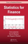
Example 5.2 (MMAR(2,2)-process).

Let the process be defined by

$\begin{array}{c}(a_1^{(1)},a_2^{(1)})=(1.1,-0.5)\\ (a_1^{(2)},a_2^{(2)})=(-1.2,-0.5)\\ {\in }_t^{(1)}\in N(0,1)\\ {\in }_t^{(2)}\in N(0,1)\end{array}$

and let the transitions between the different regimes be governed by the matrix

$P=\left(\begin{array}{cc}0.95& 0.05\\ 0.05& 0.95\end{array}\right).(5.61)$

The performance of this system is shown in Figure 5.2. The example and the figure are from Thuvesholmen [1994].

It is possible to extend the class further (MacDonald and Zucchini [1997]). Zucchini and MacDonald [2009] or Cappé et al. [2005] provides a nice overview on applications, theory and estimation methods for hidden Markov models.

Remark 5.1 (Transition mechanisms).

For various threshold models the most important difference is in the transition between the regimes:

• For SETAR the abrupt transition depends on Xt−d.
• For STAR the smooth transition depends on Xt−d.
• For HMM the transition is stochastic.

5.5.2 Models with conditional heteroscedasticity (ARCH)

The ARCH process is introduced by Engle [1982] to allow the conditional variance to change over time as a function of past observations leaving the unconditional variance constant. Hence, the recent past gives information about the one-step prediction variance.

This type of model has proven to be very useful in finance and econometrics for modeling conditional heteroscedasticity, i.e., the conditional variance is not constant, but depends on past observations. In finance the risk is expressed using the actual (conditional) variability of, for instance, the interest rate. The actual variability is called the volatility of the phenomena.

Another reason for considering models for the volatility is that this will increase the statistical efficiency of the estimates in the conditional mean model; cf. weighted least squares.

The general formulation of non-linear, conditional models is the following class of models:

$Y_t=f(Y_{t-1},{\epsilon }_{t-1},\mathrm{...},{\theta }_f)+g(Y_{t-1},{\epsilon }_{t-1},\mathrm{...},{\theta }_g){\epsilon }_t(5.62)$

where ft = f(Y, w, θf) is the conditional mean, gt = g(Y, w, θg) the conditional standard deviation and wt is white noise having unit variance.

Adding the assumption of normality, the model can be more directly expressed as

$Y_t|{ℱ}_{t-1}~N(f_t,g_t,g_t^T)(5.63)$

where ${ℱ}_t$ is the information set available at time t, and N is the multivariate probability density function with mean ft and variance $g_t{g}_t^T$.

5.5.2.1 ARCH regression model

The pure ARCH models belong to the class of conditional variance models, and the ARCH model suggested by Engle [1982] has been used in (5.46). The observation made in Engle [1982] was that volatility is clustering temporally. The basic specification of the ARCH(p) model is written as:

$\begin{array}{c}{Y}_t={\sigma }_t{w}_t\\ {\sigma }_t^2={\alpha }_0+{\alpha }_1{Y}_{t-1}^2+\mathrm{...}+{\alpha }_p{Y}_{t-p}^2,\end{array}$

where the strict white noise sequence {wt} satisfies E[wt] = 0, Var(wt) = 1while αi > 0 is a sufficient but not necessary condition to ensure positive variances. Finally, Σαi < 1 is required to ensure stationarity. Experience has shown that the number of lags, p, has to be fairly large to fit real data.

The model was used to test whether the conditional volatility depends on lagged values, i.e., if there is conditional heteroscedasticity. The tests are typically Lagrange multiplier or likelihood ratio type tests.

In the more general setup in Engle [1982] the following models are considered:

$Y_t|{ℱ}_{t-1}~F(X_t,{\beta }_t,{\sigma }_t^2),(5.64)$

where F(·,·) is some distribution (often but not exclusively Gaussian) with mean X,tβf and variance ${\sigma }_t^2,{\theta }_f={[{\alpha }^T{\beta }_f^T]}^T$ is a vector of unknown parameters, X a vector of variables included in the information set (lagged values of Y or external signals) and

$\begin{array}{cc}{\epsilon }_t=Y_t-X_t{\beta }_f,& (5.65)\\ {\sigma }_t^2={\alpha }_0+{\displaystyle \sum _{i=0}^p}{\alpha }_i{\epsilon }_{t-i}^2.& (5.66)\end{array}$

Modelling the conditional mean is important as the variance is the second moment minus the first moment squared. Ignoring the conditional mean will therefore incorrectly inflate the conditional variance.

An appealing property due to the simplicity of the ARCH(p) model is that it can be estimated using ordinary least squares, but the least square estimates won't be efficient. Maximum likelihood estimation is therefore often the estimator of choice, using the least squares estimates as initial values for the numerical maximization. The likelihood function for conditional Gaussian models can be found in Engle [1982].

An interesting interpretation of ARCH regression models mentioned by Engle [1982] is that the model for the conditional variance picks up the effect of variables not recognized or otherwise not included in the model.

The ARCH regression model is very useful in monetary theory and finance theory. Portfolios of financial assets are often assumed to be functions of the expected means and variances of the rates of return.

5.5.2.2 GARCH model

The GARCH model, proposed by Bollerslev [1986], is an extension to ARMA-like structure for the model describing the conditional variance. For the ARCH process the conditional variance is specified as a linear function of past sample variances only, whereas for the GARCH process past values of the conditional variance are used as well. The Generalized ARCH (GARCH) model is given by

$\begin{array}{cc}{\epsilon }_t|{ℱ}_{t-1}~F(0,{\sigma }_t^2)& (5.67)\\ {\sigma }_t^2=\omega +{\displaystyle \sum _{i=1}^q}{\alpha }_i{\epsilon }_{t-i}^2+{\displaystyle \sum _{i=1}^p}{\beta }_i{\sigma }_{t-i}^2& (5.68)\end{array}$

where all the coefficients (αi, βi) must be non-negative to ensure positive variances, and ${\sum }_{i=1}^p{a}_i+{\sum }_{j=1}^q{\beta }_j<1$ to preserve stability. It is also common to add additional explanatory variables to the σ2 that are expected to be highly correlated with the variance; cf. Asgharian et al. [2013].

The GARCH(p,q) can be rewritten as an ARMA process. Introduce $v={\epsilon }_t^2-{\sigma }_t^2={\sigma }_t^2(w_t^2-1)$ which is a sequence of white noise. The GARCH(p,q) process can then be written as

$(1-\psi (B)){\epsilon }_t^2=\omega +(1-\beta (B))v_t(5.69)$

where ψ (B) = α (B) + α (B). The ARMA representation of the GARCH model can be used for identification of the order of the GARCH(p,q) model. It has been argued that a GARCH(1,1) is often sufficient for most data sets (Hansen and Lunde [2005]).

There are plenty of non-linear GARCH models (Bollerslev [2008]). Many of these are using the connection between ARMA and GARCH models, extending the ARMA structure by features originating from SETAR or STAR models.

Extending to the GARCH regression model is similar to the extension for the ARCH model

$Y_t|{ℱ}_{t-1}~F(X_t{\beta }_f,{\sigma }_t^2).(5.70)$

It has been argued that a GARCH(1,1) is sufficient; cf. Hansen and Lunde [2005]. They test a large number of alternative specifications and find, after compensating for the asymmetrical test procedure, that they are unable to reject the GARCH(1,1) in favor of more advanced ARCH/GARCH models.

5.5.2.3 EGARCH model

The GARCH model has a major limitation in that it is symmetric, i.e., it doesn't predict the volatility to behave differently depending on the sign of εt, contrary to empirical observations on real data.

Another problem with the GARCH model is the requirements on the parameters, making the numerical optimization difficult. These arguments were addressed in the introduction of the EGARCH model in Nelson [1991], specified as

$\begin{array}{cc}{\epsilon }_t=w_t{\sigma }_t,& (5.71)\\ {\sigma }_t=exp\left(\frac{1}{2}{h}_t\right),& (5.72)\\ h_t=\omega +{\displaystyle \sum _{i=1}^p}{\alpha }_i{w}_{t-1}+{\displaystyle \sum _{i=1}^q}{\beta }_i{h}_{t-i}.& (5.73)\end{array}$

The EGARCH-process addresses the symmetry problems and does also impose less restrictions on the parameters, as the exponent of the conditional variance equation is an ARMA-process.

5.5.2.4 FIGARCH model

One of the more remarkable stylized facts is the dependence in squared or absolute returns (Section 1.3.7). Long range dependence in ordinary time series is often modeled using ARFIMA models (Granger and Joyeux [1980]). Their idea is introduce a fractional differentiation of the ARIMA model in Section 4.4.2 according to

$\varphi (B){(1-B)}^d{Y}_t=\theta (B){\epsilon }_t,(5.74)$

where d is some number between 0 and 1. This leads to a model that sits somewhere in between the stationary ARMA model and the non-stationary ARIMA model. They also show that the variance of the resulting process is finite if d < 1/2. Requirements for the volatility process to imposed positivity of the process can be found in Conrad and Haag [2006].

Similar ideas were employed on GARCH models in Baillie et al. [1996], Bollerslev and Ole Mikkelsen [1996], as the GARCH model can be written as an ARMA model (Equation (5.69)). Recall the ARMA representation of the GARCH model

$(1-\psi (B)){\epsilon }_t^2=\omega +(1-\beta (B))v_t(5.75)$

while the IGARCH representation is given by

$\Phi (B)(1-B){\epsilon }_t^2=\omega +(1-\beta (B))v_t(5.76)$

where Φ(B) = (1 − α(B) − β(B))(1 − B)−1 being of order m − 1 with m = max(p, q). The FIGARCH is defined by replacing the first-order differentiation by a fractional differentiation

$\Phi (B){(1-B)}^d{\epsilon }_t^2=\omega +(1-\beta (B))v_t(5.77)$

with the process having finite variance if −.5 < d < 0.5. Fractional differentiation can be expressed by the hypergeometric function

${(1-B)}^d={\displaystyle \sum _{k=0}^{\infty }\frac{\Gamma (k-d)}{\Gamma (k+1)\Gamma (-d)}{B}^k}.(5.78)$

The implications of the fractional integration in terms of memory of the process are analyzed in Davidson [2004].

5.5.2.5 ARCH-M model

Several extensions of the basic ARCH model are possible. In Engle et al. [1987] the ARCH model is extended to allow the conditional variance to affect the mean. In this way changing conditional (co-)variances directly affect, for instance, the expected return; cf. CAPM.

The models are called ARCH-in-Mean or ARCH-M models. The ARCH-M is obtained by a slight modification of Equation (5.63)

$Y_t|{ℱ}_{t-1}~F(X_t{\theta }_f+\delta {\sigma }_t^2,{\sigma }_t^2)(5.79)$

where the conditional variance σt2 is given by the ARCH model. It is possible to generalize the ARCH-M models by replacing the ARCH model by arbitrary conditional variance models. Additionally, other mean specifications have also been suggested such as

$Y_t|{ℱ}_{t-1}~F(X_t{\theta }_f+\delta {\sigma }_t,{\sigma }_t^2)(5.80)$

or

$Y_t|{ℱ}_{t-1}~F(X_t{\theta }_f+\delta \log ({\sigma }_t^2),{\sigma }_t^2)(5.81)$

(Engle et al. [1987]).

5.5.2.6 SW-ARCH model

A further extension of the ARCH models is the switching ARCH model. The idea of the switching ARCH model is to use a combination of different ARCH models. One possible parametrisation is given by

${\epsilon }_t=\sqrt{g(S_t)}{\sigma }_t{w}_t,(5.82)$

${\sigma }_t^2={\alpha }_0+{\displaystyle \sum _{i=1}^p{(\alpha {(S_t)}_{t-1}{\epsilon }_{t-i})}^2}(5.83)$

where St is the state of a hidden Markov chain taking K different states, and g(St) is a constant taking different values depending on St. The model can be interpreted as an extension of the ordinary ARCH(p) process by using different ARCH(p) processes for each state of the market.

Switching models are significantly more difficult to estimate than ordinary (G)-ARCH models due to the large number of additional parameters and complex likelihood function (see e.g. Henricsson [2002]), but it can be argued that the states can be interpreted as states of the market, e.g., recession or boom, giving an increased understanding of data.

5.5.2.7 General remarks on ARCH models

The performance of ARCH-like models can often be improved using a combination of the following three different strategies:

1. The AR or ARMA structure of the conditional variance can be extended by introducing external signals (ARX or ARMAX), e.g., it is commonly believed that the trading volume can be used to predict the volatility.

2. The distribution of wt does not have to be Gaussian. In fact, it is often better to use the t-distribution or the generalized error distribution, the latter being specified (having zero mean and unit variance) as

   $f(x)=\frac{v\exp \left(-\frac{1}{2}{|\frac{x}{\lambda }|}^v\right)}{\lambda 2^{(v+1)/v}\Gamma (1/v)},(5.84)$

   where λ is a constant given by

   $\lambda ={\left\{\frac{2^{-(2/v)}\Gamma (1/v)}{\Gamma (3/v)}\right\}}^{1/2}.(5.85)$

   Other alternatives include the variance gamma or the normal inverse Gaussian (henceforth called the NIG) distribution. The NIG distribution is a Gaussian mean variance mixture model (Barndorff-Nielsen [1977]), and has been popular in econometrics (Jensen and Lunde [2001], Kiliç [2007]) as well as in the option valuation literature (Cont and Tankov [2004] and Definition 7.11). The probability density function is given by

   $f_{NIG}(x)=\frac{\alpha \delta K_1(\alpha \sqrt{{\delta }^2+{(x-\mu )}^2)}}{\pi \sqrt{{\delta }^2+{(x-\mu )}^2}}{e}^{\delta \gamma +\beta (x-\mu )},(5.86)$

   where μ is a location parameter, a controls the tail heaviness, β is an asymmetry parameter and δ is a scale parameter. Finally, K1 is a modified Bessel function of the second kind.

3. Introducing a non-linear influence of old values of εt−i to account for the the asymmetric response of volatility shocks. This can be done by replacing lagged values of, e.g., ${\epsilon }_t^2$ by a function f(εt−i/σt−i). The modified EGARCH model would then be specified as

   ${\epsilon }_t={\sigma }_t{w}_t(5.87)$

   ${\sigma }_t=\exp \left(\frac{1}{2}{h}_t\right)(5.88)$

   $h_t={\alpha }_0+{\displaystyle \sum _{i=1}^{p}f(w_{t-i})+}{\displaystyle \sum _{i=1}^q{\beta }_i{h}_{t-j}}(5.89)$

   where f(wt−i) = λ(|wt−i| − E [|wt−i|]) + γwt−i. The response will then depend on the sign of wt−i, allowing for different response to good and bad news.

   A related modification is the Glosten-Jagannathan-Runkle (GJR) GARCH model (Glosten et al. [1993]), where the conditional volatility is given by

   ${\sigma }_t^2={\alpha }_0+{\displaystyle \sum _{t=1}^q({\alpha }_i{\epsilon }_{t-1}^2+{\gamma }_i{l}_{\{{\epsilon }_{t-i}<0\}}{\epsilon }_{t=i}^2)}+{\displaystyle \sum _{i=1}^p{\beta }_i{\sigma }_{t-i}^2}.(5.90)$

   Estimating a positive γi parameter means that additional volatility is found due to bad news.

5.5.2.8 Multivariate GARCH models

The are many multivariate GARCH models; see Silvennoinen and Teräsvirta [2009b], for a review. These are defined similarly to the univariate models

$r_t=H_t^{1/2}{\eta }_t,(5.91)$

where ηt, is an iid zero mean, unit covariance random vector. The log-likelihood (when η is a Gaussian vector) for these models is given by

${\ell }_t(\theta )=-\frac{1}{2}{\displaystyle \sum _{t=1}^T\ln |\det (2\pi H_t)|-\frac{1}{2}{\displaystyle \sum _{t=1}^T{r}_t^T{H}_t^{-1}{r}_t}}.(5.92)$

It is rarely possible to write down closed form expressions for the parameter estimates. Equation (5.92) must therefore be maximized using numerical optimization. Many models are overparametrized from a practical point of view, which is why the CCC and DCC models (more on those below) are popular.

The first multivariate GARCH model was the VEC-GARCH model (Bollerslev et al. [1988]), which is a straightforward generalization of the univariate version. The model, for a N-dimensional problem, is given by

$\text{vech}(H_t)=c+{\displaystyle \sum _{j=1}^p{A}_j\text{vech}(r_{t-j}{r}_{t-j}^T)+{\displaystyle \sum _{j=1}^q{B}_j\text{vech}(H_{t-j})}}(5.93)$

where the vech(·) operator stacks the columns of the lower triangular part of the matrix. Sufficient conditions for strictly positive variances are rather restrictive, and the model is also haunted by the shear number of parameters in it. It can be shown that the dimension of the Ai and Bi matrices is N(N + 1)/2 × N(N + 1)/2 and hence that the total number of parameters is given by (p + q)(N(N + 1)/2)2 + N(N + 1)/2.

A restricted version of the VEC-GARCH model is the BEKK model (Engle and Kroner [1995]). The number of parameters in this model is lower than for the VEC-GARCH model, and the conditional variances are always positive by construction. The conditional co-variance is given by

$H_t=C{C}^{\prime }+{\displaystyle \sum _{j=1}^q{\displaystyle \sum _{k=1}^K{A}_{kj}^T{r}_{t-j}{r}_{t-j}^{T}Akj}+{\displaystyle \sum _{j=1}^p{\displaystyle \sum _{k=1}^K{B}_{kj}^T{H}_{t-j}{B}_{kj},}}}(5.94)$

where Akj, Bkj and C are N × N matrices, and C is lower triangular. The estimation is still rather complicated as the number of parameters is (p + q)KN2 + N(N + 1)/2.

A simpler model is the Constant Conditional Correlation-GARCH model due to Bollerslev [1990]. Here the conditional covariance matrix is defined as

$H_t=D_{t}O{D}_t(5.95)$

where $D_t=diag(h_{1t}^{1/1},...,h_{Nt}^{1/2})$ and P is a positive definite correlation matrix.

The models for the processes rit are given by univariate models, which, in case of GARCH models, leads to the vector conditional variance process

$h_t=\omega +{\displaystyle \sum _{j=1}^q{A}_j{r}_{t-j}\odot r_{t-j}}+{\displaystyle \sum _{j=1}^p{B}_j{h}_{t-j}},(5.96)$

where ω is a N × 1 vector, A and B are N × N matrices and ⊙ is element-wise multiplication.

The CCC-GARCH is often considered to be too simple, as it is unable to capture varying correlations. The Dynamic Conditional Correlation-GARCH (see Engle [2002]) replaces the fixed correlation matrix with a dynamics matrix. Start by defining the matrix Qt as

$Q_t=(1-a-b)S+a{\epsilon }_{t-1}{\epsilon }_{t-1}^T+b{Q}_{t-1}.(5.97)$

The constants a and b are positive numbers satisfying a + b < 1, S is the unconditional correlation matrix of the standardized errors e and the initial condition Q0 is some positive definite matrix. This matrix is rescaled to obtain a dynamic correlation matrix according to

$P_t={(I\odot Q)}^{-1/2}Q{(I\odot Q)}^{-1/2}.(5.98)$

The additional flexibility is inexpensive from a computational point of view as only two (a and b) new parameters were added. Several extensions of the DCC-GARCH have been proposed (see e.g. Cappiello et al. [2006] and references therein).

Another extension is the Smooth Transition Conditional Correlation-GARCH suggested by Silvennoinen and Teräsvirta [2005, 2009a]; cf. Section 5.5.1.4. Their idea is to use a smooth transition between fixed correlations

$P_t=(1-G(s_t))P^{(1)}+G(s_t)P^{(2)},(5.99)$

where P(1), P(2) are correlation matrices and G(·) is some smooth transition function. A particularly nice feature with the STCC-GARCH model is the possibility to test for smooth transition effects, by using a Lagrange multiplier test, starting from the standard CCC-GARCH (Silvennoinen and Teräsvirta [2009a]).

5.5.3 Stochastic volatility models

A different class of models describing volatility changing over time is the class of stochastic volatility models. The important difference between stochastic volatility models and the class of ARCH models is that the stochastic volatility models specify the volatility as a latent or unobservable process. This could be a significant advantage (but it is not for free as we will see soon) as the volatility at time t + 1 is not completely determined at time t. This matters when there are unexpected shocks, such as terrorist attacks.

A simple stochastic volatility model (Taylor [1982]) is given by

$Y_t=\exp (V_t/2)w_t,(5.100)$

$V_t=\alpha +\beta V_{t-1}+e_t,(5.101)$

where wt and et are white noise having unit variance. The class of stochastic volatility models can be generalized to continuous time models, where they are being used to derive improved option pricing formulas.

Parameters in discrete time stochastic volatility models can be approximately estimated using Kalman filters (Quasi-Maximum Likelihood), cf. Chapter 14, or using Monte Carlo methods, like MCMC or Sequential Monte Carlo methods (Lopes and Tsay [2011]).

The stochastic volatility can be transformed into a nicer problem by considering ${\xi }_t=\log (Y_t^2)$. This leads to

${\xi }_t=\log (\exp (V_t))+\log (w_t^2),(5.102)$

$V_t=\alpha +\beta V_{t-1}+e_t,(5.103)$

which is a linear model. The downside is that $\log (w_t^2)$ is non-Gaussian. It can be shown that $E[\log (w_t^2)]\approx -1.27$ and $\mathrm{Var}[\log (w_t^2)]={\pi }^2/2$. Using a Kalman filter to estimate the parameters is suboptimal (it is not a likelihood method), but the estimates will still be consistent. The Quasi-ML estimates are therefore useful as starting values for a likelihood based method, while modern Monte Carlo methods can provide an approximate maximum likelihood estimate; see Section 14.10 or (Cappé et al. [2005]).

Remark 5.2

Recall that for a normal distributed stochastic variable, X ∈ N(μ, υ2), it holds that

$\begin{array}{llll}E[X]\hfill & =\hfill & \mu \hfill & 5.104\hfill \\ E[X^2]\hfill & =\hfill & {\mu }^2+{\sigma }^2\hfill & 5.105\hfill \\ E[X^3]\hfill & =\hfill & {\mu }^3+3\mu {\sigma }^2\hfill & 5.106\hfill \\ E[X^4]\hfill & =\hfill & {\mu }^4+6{\mu }^2{\sigma }^2+3{\sigma }^4\hfill & 5.107\hfill \\ E[X^5]\hfill & =\hfill & {\mu }^5+10{\mu }^3{\sigma }^2+15\mu {\sigma }^4\hfill & 5.108\hfill \\ E[X^6]\hfill & =\hfill & {\mu }^6+15{\mu }^4{\sigma }^2+45{\mu }^2{\sigma }^2+15{\sigma }^6\hfill & 5.109\hfill \\ E{[X-E[X])}^n]\hfill & =\hfill & {\mu }^{2n}(2n-1)!!\hfill & 5.110\hfill \end{array}$

for n ∈ ℕ where n!! denotes the double factorial, i.e., the product of every odd number from n to 1.

Recall also that Y = exp(X) is lognormally distributed LN(μ, υ2), and that

$\begin{array}{llll}E[Y]\hfill & =\hfill & \exp (\mu +{\sigma }^2/2)\hfill & (5.111)\hfill \\ E[Y^n]\hfill & =\hfill & \exp (n\mu +n^2{\sigma }^2/2)\hfill & (5.112)\hfill \\ \mathrm{Var}[Y]\hfill & =\hfill & E[{(Y-E[Y])}^2]=\exp (2\mu +{\sigma }^2)(\exp ({\sigma }^2)-1)\hfill & (5.113)\hfill \end{array}$

for n ∈ ℕ.

5.6 Model identification

Model identification of non-linear models is almost an art, as the number of possible models grows rapidly with increasing dimension of the parameter vector. The mainstream approach to model identification is to discover the dominant features in data without going into specific models.

This is done in Nielsen and Madsen [2001] and Lindström [2013a] where it is shown how a linear model can be compared to a general non-linear model, defined either as a non-parametric model (Nielsen and Madsen [2001]) or semiparametric model (Lindström [2013a]). The latter even admits testing in terms of adjusted F-tests.

Modern variable selection techniques, such as Lasso, LARS or elastic net (Hastie et al. [2009]), make it possible to estimate and shrink complex models without thinking too much about the exact model structure. This presents a different approach as identification and model fitting procedure is merged into a single step.

5.7 Prediction in nonlinear models

Under exactly the same conditions as for linear models (see Madsen [2007]) the optimal prediction is given as the conditional mean, i.e.,

${\widehat{Y}}_{t+k|t}=E[Y_{t+k}|{ℱ}_t](5.14)$

where ℱt is the information set at time t.

One of the noticeable differences is, however, that the predictor is in general not linear in the elements of the information set. This is illustrated in the following simple example.

Example 5.3 (Prediction).

Consider the first-order model

$Y_t=f(Y_{t-1},\theta )+{\epsilon }_t(5.115)$

where {εt} is a strict white noise.

For this model the optimal predictor is

$E[Y_{t+1}|{\psi }_t]=E[Y_{t+1}|Y_t=y]=f(y,\theta )(5.116)$

where the fact that the model is a first-order Markov model has been used in the first equality.

The important difference between white noise and a strict white noise is illustrated in the next example.

Example 5.4.

Consider the process

$Y_t={\epsilon }_t+\theta {\epsilon }_{t-1}{\epsilon }_{t-2}(5.117)$

where {εt} is strict white noise.

The one-step predictor is

${\widehat{Y}}_{t+1|t}=\theta {\epsilon }_{t-1}{\epsilon }_{t-2}.(5.118)$

Let us for illustration consider the autocovariance function for {Yt}

$\begin{array}{llll}{\gamma }_k\hfill & =\hfill & E[y_t{Y}_{t+k}]=E[{\epsilon }_t{\epsilon }_{t+k}+\theta {\epsilon }_{t-1}{\epsilon }_{t-2}{\epsilon }_{t+k}]\hfill & (5.119)\hfill \\ \hfill & +\hfill & \theta {\epsilon }_t{\epsilon }_{t+k-1}{\epsilon }_{t+k-2}+{\theta }^2{\epsilon }_{t-1}{\epsilon }_{t-2}{\epsilon }_{t+k-1}{\epsilon }_{t+k-2}]\hfill & (5.120)\hfill \\ \hfill & =\hfill & 0fork\ne 0,\hfill & (5.121)\hfill \end{array}$

i.e., {Yt} is white noise. Hence, a non-linear predictor has to be used in order to use the information set for prediction.

5.8 Applications of nonlinear models

5.8.1 Electricity spot prices

Hidden Markov models are frequently used when modelling the electricity spot price (these models are often called Independent Spike Models; see Huisman and Mahieu [2003], Janczura and Weron [2010], Regland and Lindström [2012], Lindström and Regland [2012]) as these are often extremely volatile. Renewable energy (e.g. wind power) is less predictable than classical sources of energy. Surplus or lack of energy leads inevitably to large temporal variations in the price.

It is well known that electricity spot prices are mean-reverting and heteroscedastic, and there are also seasonal effects (yearly, weekly and daily) and jumps (Escribano et al. [2011]). The independent spike models provide a simple and very efficient solution to this problem by modelling the spread between the spot price and the forward price, as the forward price is essentially a robust, low-pass filtered version of the spot price (Figure 5.3).

The spread accounts for virtually all seasonality, but there are still bursts of volatility. The logarithm of the spot, yt, was modeled in Regland and Lindström [2012] using a HMM regime switching model with three states, a normal state with mean-reverting dynamics, a spike (upward jumps) state and a drop (downward jumps) state. This is mathematically given by:

$\begin{array}{c}\Delta y_{t+1}^{(B)}=\alpha \left({\mu }_t-y_t^{(B)}\right)+\sigma {\epsilon }_t\\ y_{t+1}^{(S)}=Z_{s,t}+{\mu }_t,Z_s~LogN({\mu }_s,{\sigma }_s)\\ y_{t+1}^{(D)}=-Z_{D,t}+{\mu }_t,Z_D~LogN({\mu }_D,{\sigma }_D)\end{array}$

where μt is the logarithmic month ahead forward price.

The regimes are switching according to a Markov chain Rt = {B, S, D} governed by the transition matrix

$\Pi =\left[\begin{array}{ccc}1-{\pi }_{BU}-{\pi }_{BD}& {\pi }_{BS}& {\pi }_{BD}\\ {\pi }_{SB}& 1-{\pi }_{SB}& 0\\ {\pi }_{DB}& 0& 1-{\pi }_{DB}\end{array}\right].$

The resulting fit of the model is presented in Figure 5.4, where we see that the regime switch captures the bursts well.

5.8.2 Comparing ARCH models

The performance of different models for conditional variance was evaluated in Henricsson [2002]. Different ARCH(p), GARCH(p,q) and SW-ARCH (with two regimes) models were evaluated on the Swedish stock index Affärsvärldens generalindex from 1980 to 2001 using a moving window of 4 years of data to estimate the models and the following year to evaluate the forecasting performance. Some observations generated by the study were:

• The standardized residuals are not Gaussian, but are more heavy-tailed, possibly even student-t distributed.
• It is important to include a term in the volatility equation that captures the asymmetric effect of lagged innovations εt−i.
• The persistence in volatility can only be captured in a satisfactory way using the GARCH model, although the improvement using SW-ARCH over an ordinary ARCH model is significant. Could a SW-GARCH capture both the persistence and the switching regimes?

Recent studies (Nystrup et al. [2014]) indicate that as many as four states are needed to to model equity returns, as two or three state regime switching models are unable to capture both the conditional distribution and the dependence structure found in market data.

5.9 Problems

Problem 5.1

Consider a SETAR(3;1;1,1,2) model for a univariate time series Yt, where R1 =] −∞, 0], R2 =]0,15] and R3 =]15, ∞[.

1. Specify the thresholds and the delay parameter.
2. Write down the model.
3. Does the model pertaining to the second regime R2 need to be stable for the complete model to be stable?

Problem 5.2

Consider a STAR(2) with a delay parameter of 1.

1. Write down the model.
2. What is the major difference between SETAR and STAR models?

Problem 5.3

It is common to observe burst-like phenomena in financial time series, which may be due to governmental interventions in the market, attacks on some currency in the foreign exchange markets, the effects of earthquakes in California and other unpredictable phenomena. Such phenomena may be described by bilinear models.

1. Write down the bilinear model BL(2,0,1,1).
2. Write down the autocovariance function for this particular model.
3. Is it possible to uniquely identify a BL(2,0,1,1) model using this autocovariance function?

Problem 5.4

Consider the ARCH model (5.46) as a model of interest rates rt.

1. Which important characteristics do the ARCH models have compared to linear ARMA models?
2. Write down an ARCH(3) model.

Problem 5.5

Consider the ARCH(1) process

$\begin{array}{l}{X}_t=\sqrt{h_t}{Z}_t\\ h_t=a_0+a_1{X}_{t-1}^2.\end{array}$

1. Calculate the p'th moment of Xt for p ∈ ℕ.
2. Can you use information about the moments to estimate parameters?
3. What about GARCH and EGARCH models?

Problem 5.6

Consider the stochastic volatility model

$\begin{array}{c}{X}_t=\exp \{V_t/2\}{Z}_t,\\ V_t=a_0+a_1{V}_{t-1}+e_t,\end{array}$

and assume Z and e are zero mean, unit variance independent random variables.

1. Calculate mean, variance and covariance of Vt.

2. Calculate $E[X_1^2]$.

   Hint: We can write the model as

   $\ln X_t^2=\ln Z_t^2+V_t,(5.122)$

   where $E[\ln Z_t^2]=-(\ln (2)+\gamma )\approx -1.27$ and $\mathrm{Var}[\ln Z_t^2]={\pi }^2/2$.

3. Calculate the autocovariance

   $Cov(\ln X_t^2,\ln X_{t+k}^2)=rv(k)+\frac{{\pi }^2}{2}1\{k=0\},(5.123)$

   where 1{k=0} is an indicator function, being 1 if k = 0 and zero otherwise.