
Chapter 3
Discrete time finance
This chapter will describe discrete time models in order to introduce the reader to some of the basic concepts to be used in subsequent chapters on continuous time. The theory in discrete time is simpler as the proofs only require linear algebra.
In this chapter we shall consider simple models of security markets and describe the basic principles of valuation of contingent claims (e.g., options, futures). The key idea behind valuation in markets with uncertainty is the notion of absence of arbitrage. Roughly speaking, an arbitrage is a situation where an investor, through buying and selling securities, takes a “position” in the market which has zero net cost and which guarantees 1) no losses in the future and 2) some chance of making a profit. In a model free of arbitrage such investments are not possible.
3.1 The binomial one-period model
Consider a financial market with two securities, a stock and a bond, and two time points t = 0 and t = 1. The bond is a riskless asset with initial price B0, and price (1 + r)B0 at time t = 1, where r > 0 is the deterministic constant interest rate and (1 + r)−1 is the discounting factor. The initial stock price is given by S0 and the price at time t = 1 is assumed to be unknown. At time t = 1 the market can be in either of two states. With probability p the stock price will be S11 associated with state 1 (the upper index indicates the state), and with probability 1 − p the stock price is S21 at time t = 1.
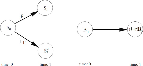
Suppose an investor is interested in a contract, e.g., an option which pays c1 if state 1 is realized and c2 if state 2 is realized. What should such a contract cost in the one-period financial market consisting of a stock and a bond? One suggestion would be to price the contract as the expected value of future payoffs, discounted by the factor (1 + r)−1. Let V denote the price of the contract. Then
ˆV=(1+r)−1E[C]=(1+r)−1(pc1+(1−p)c2)·(3.1)
We shall, however, see that this is not correct, at least not in the naive form; cf. Harrison and Pliska [1981], Biagini and Cont [2006].
Consider instead a general portfolio (ϕ,ψ)∈ℝ2, consisting of ϕ units of the stock and ψ units of the bond. The price of that portfolio at time t = 0 is ϕS0+ψB0
At time t = 1 the value of that portfolio would be ϕS11+ψ(1+r)B0 in state 1 and ϕS21+ψ(1+r)B0 in state 2. To find the correct price of the contract we could choose the portfolio (ϕ, ψ) in a way that yields c1 in state 1 and c2 in state 2. The principle of buying a portfolio with the same cash flow/payoff as a contract is called replication. By solving the linear equations
ϕS11+ψ(1+r)B0=c1(3.2)
ϕS21+ψ(1+r)B0=c2(3.3)
the following portfolio is obtained
ϕ=c2−c1S21−S11(3.4)
ψ=1(1+r)B0(c2−(c2−c1)S21S21−S11)·(3.5)
If this portfolio is bought, the payoff at time t = 1 would be cj in state j = 1,2. The price ˜V of the portfolio at time t = 0 is
˜V=ϕS0+ψB0=S0(c2−c1S21−S11)+1(1+r)(c2−(c2−c1)S21S21−S11)·(3.6)
This is an other candidate to the price of the contract which differs from (3.1), and this is the correct price as we shall see.
Consider some other market maker offering to buy or sell the contract for a price P less than ˜V. Anyone could buy the contract in arbitrary quantity, and sell the portfolio (ϕ, ψ) above to replicate it. At time t = 1 the value of the contract would exactly cancel the value of the portfolio, whatever the stock price would be — thus this set of trades carries no risk. But the trades were carried out with a profit of ˜V−P per unit of contract. By buying arbitrary amounts anyone could make arbitrary risk-free profits, so P would not have been a rational/fair price for the market maker to quote.
Similarly if the market maker quotes a price P greater than ˜V, anyone could again make arbitrary risk-free profits. Hence the price ˜V is the rational/fair price for that contract. In the next section a more general1 model will be considered, which includes this model as a special case.
3.2 One-period model
The model considered in this section is the simplest possible model of a security market with uncertainty — the Arrow-Debreu model. We assume that there are N securities with the initial price vector S0=(S10,S20,...,SN0)T, which can be held in any positive or negative real number by any investor. An investor is said to hold a short position of a given security if he or she has a negative amount of that security, and the position is long if the investor has a positive amount. The security prices S0 are known at time t = 0 while the future prices S1 are unknown at time t = 0. It is assumed that the market can be in M different states ωi at time t = 1, and the security prices at time t = 1 can be represented by the cash-flow matrix D ∈ ℝN × M as follows
D=[S11(ω1)S11(ω2)⋯S11(ωM)S21(ω1)S21(ω2)⋯S21(ωM)⋮⋮⋱⋮SN1(ω1)SN1(ω2)⋯SN1(ωM)]=[S1(ω1)S1(ω2)⋯S1(ωM)](3.7)
where ωj is an outcome from the finite sample space Ω = {ω1, ω2,..., ωM} and S1(ωj) ∈ ℝN is the price vector at state j. Thus if the uncertainty in the market generates the outcome ωj, the stock price will be S1 (ωj).
The jth column of D is the price vector S1 (ωj) ∈ ℝN associated with state j and the ith row is the possible payoffs which are associated with holding one unit of security j.
A portfolio of securities is represented by a column vector h = (h1, h2,...,hN)T, i.e., (h ∈ ℝN), where hi denotes the number of securities of type i bought at time t = 0. The portfolio h is defined on ℝN, i.e., h ∈ ℝN. This implies that the investor is allowed both to go short in any security and own a noninteger number of any securities (e.g., 0.3). Assume, e.g., that h1=−√2. This means that at time t = 0 you get −√2S10 and at time t = 1 you owe −√2S11(ω), which is a stochastic variable.
The wealth process Vt (h) is defined as
Vt(h)=N∑ihiSit=hTStfort=0,1(3.8)
and it equals the value of a given portfolio as a function of the time (t = 1,2), of the initial price vector S0, and of the outcome of the stochastic variable S1(ω).
Definition 3.1 (Arbitrage in discrete time).
An arbitrage portfolio is a portfolio h such that hT S0 = 0 and
hTD·j≥0forall1≤j≤M(3.9)hTD·j>0forsome1≤j≤M(3.10)
where D·j denotes the jth column of D.
This means that an arbitrage portfolio is a zero investment portfolio (at t = 0) where losses are impossible (at time t = 1) and there is a positive probability to make a profit (at time t = 1), provided that all ωj > 0.
3.2.1 Risk-neutral probabilities
As stated in the introduction, the value of a given security is in general not given by the discounted expected value of future cash flows. In the following we shall show that the right price of a security, in the sense of no arbitrage opportunities, is the discounted expected value of future cash flows. However, the expectation should be computed with respect to an other probability measure (possibly non-unique) called the risk-neutral probabilities q, which in general differ from the objective probabilities p.
Theorem 3.1 (State price vector).
If there exists a vector of strictly positive numbers q ∈ q∈ℝM++
q=(q1,q2,...,qM)T,(3.11)
called a state price vector, such that
S0=Dq=M∑j=1qjD·j,(3.12)
then no arbitrage portfolios exist. Conversely, if there are no arbitrage portfolios, there exists a state price vector q with positive entries satisfying (3.12).
Proof. See Duffie [1996].
The theorem says that the initial price vector and the cash-flow matrix D must satisfy certain conditions in an arbitrage-free model. Given a state price vector π for the pair (D, S0), let q0=∑Mi=1qi, and for any state j, let ˆqj=qj/q0. The vector ˆq=(ˆq1,ˆq2,...,ˆqM)T has positive elements and the sum is 1 by construction; hence, it can be interpreted as a probability distribution.
By inserting qj=ˆqjq0 in (3.12) we obtain
Si0=M∑j=1q0ˆqjDij=q0M∑j=1ˆqjDij=q0Eℚ[Di·](3.13)
where Eℚ[·] denotes the expectation operator with respect to the risk-neutral probabilities.
Suppose there exists an investment opportunity which guarantees a riskless payoff of 1 USD at time t = 1. In terms of the model the payoff of this riskless investment can be represented as a vector (1,1,..., 1) in ℝM. According to Theorem 3.1 the value of such an investment must be qj = ∑Mjqj=q0. Since a bond basically is a security that pays a certain amount — say 1 USD without any loss of generality — at the expiry date (t = 1), the price of a bond in this one-period model is q0. We call q0 the discounting factor because it tells us how much 1 USD at time t = 1 is worth today t = 0.
Equation (3.13) states that the fair price of a security in a model free of arbitrage is the discounted expected payoff at time (t = 1), where the risk-neutral probabilities are used in the expectation. The change from the objective probabilities p to the risk-neutral “probabilities” q thus incorporates the discounting factor q0, as well as the real risk-neutral probabilities ˆq.
Remark 3.1.
We will see in the corresponding chapter on continuous-time models that a slightly more general formulation is used. The definition there is that a risk-neutral probability measure is a probability measure such that ratios of traded assets are martingales
S0B0=Eℚ[S1B1]·(3.14)
This definition will be helpful when valuing, e.g., interest rate derivatives.
3.2.2 Complete and incomplete markets
In the binomial model (with two states) presented in the beginning of this chapter any vector of future cash flows, c = (c1, c2), can be replicated in terms of a portfolio of a stock and a riskless bond. This property can be generalized to the setting of N securities and M states.
Definition 3.2 (Complete market).
A securities market is said to be complete if, for any cashflow vector c = (c1, c2,..., cM), there exists a portfolio h = (h1, h2, ..., hN)T of traded securities, which has a cashflow cj in state j, for all 1 ≤ j ≤ M.
Remark 3.2.
Market completeness is therefore equivalent to the existence of a solution h ∈ ℝN to the linear equations
hTD=c(3.15)
for any c ∈ ℝM, where D is the cashflow matrix defined in (3.7). From linear algebra it is well known that this property is satisfied ifand only if
rank(D)=m(3.16)
which is equivalent to saying that the rows of the matrix D span the entire ℝM space.
Remark 3.3.
A necessary condition for market completeness is that the number of traded securities must be at least as large as the number of states.
Proposition 3.1.
Suppose that the market is complete and the model is free of arbitrage. Then there exists a unique set of state prices (π1, π2,..., πM) and hence a unique set of risk-neutral probabilities ˆπ1,ˆπ2,...,ˆπM. Conversely, if there exists a unique set of state prices, then the market is complete.
Proof. Market completeness implies that the price of a contingent claim which pays $1 in state j and 0 otherwise is determined for all j. Therefore, there can be at most one set of state prices. Hence, if they exist they are unique.
The converse statement, that if there exists a unique state price vector (with strictly positive elements) then the market is complete, is proved by a contradiction argument. Assume the market is not complete, then rank(D) < M. From linear algebra, we know that the matrix D must have a non-empty nullspace, i.e., there exists a vector λ = (λ1, λ2,..., λM) such that
Dλ=0·
Using the no arbitrage relation (3.12) we obtain
S0=D(q+ρλ)
for all real numbers ρ. Since the entries of q are strictly positive, we can choose ρ sufficiently small such that qj + ρλj is positive for all j. Therefore we have constructed a new state price vector, contradicting the hypothesis. We conclude that in a market free of arbitrage, uniqueness of state prices implies that the market is complete.
The concept of completeness is a convenient idealization of the behaviour of securities markets. However markets — with many possible price structures satisfying the no-arbitrage condition — are the rule rather than the exception.
Example 3.1 (The trinomial model).
By adding one more state to the binomial model in Section 3.1 we obtain the so-called trinomial model, which is an incomplete market since the cashflow matrix D is 2 × 3. Due to the fact that the state prices are not unique, the price ofcontingent claims can not in general be determined uniquely.
Assuming that there is a riskless bond on the financial market, with a deterministic rate r and a value of one at time t = 1, and assuming no arbitrage then we get from (3.13) that
11+r=q1+q2+q3Bondprice(3.17)
S0=S11q1+S21q2+S31q3Stockprice (3.18)
S11<S21<S31.(3.19)
Admissible sets of state prices π must satisfy Equations (3.17)—(3.18) and must have strictly positive entries. By subtracting (3.18) from (3.17) we obtain
0=(1+r−S11S0)q1+(1+r−S21S0)q2+(1+r−S31S0)q3.(3.20)
Since q is strictly positive the equation above can only be fulfilled if
S11S0<1+r<S31S0.(3.21)
With this condition the model is free of arbitrage, and the set of admissible state prices can be visualized as a line segment corresponding to the intersection of the planes described by (3.17) and (3.18) in the positive quadrant ℝ3++.
Since the state prices are strictly positive in all coordinates, the extreme values at the line segments are
q1=S31S0−(1+r)(1+r)(S31S0−S11S0),q2=0,q3=(1+r)−S11S0(1+r)(S31S0−S11S0),(3.22)
and
q1=0,q2=S31S0−(1+r)(1+r)(S31S0−S21S0),q3=(1+r)−S12S0(1+r)(S31S0−S21S0)(3.23)
if S21S0≤(1+r), or
q1=S21S0−(1+r)(1+r)(S21S0−S11S0),q2=(1+r)−S11S0(1+r)(S21S0−S11S0),q3=0,(3.24)
if S21/S0>(1+r).
Due to the fact that the model is incomplete, the price of derivatives cannot be determined uniquely. However, since the set of admissible state prices is the line segment mentioned above, bounds on the value of derivatives can be calculated. Since the value of the derivative is a linear function, and the line segment is an open convex set, an infimum and supremum of the price can be found. To illustrate this, consider the case of a call option on the basic security S, with strike price K. Assume that S21<K<S31. Then the cash flows for this option are S31−K in state 3 and 0 in state 1 and 2. Its no-arbitrage value is C=π3(S31−K).According to the extreme values of the admissible line segment the upper bound for the call option is
C+=π3(s31−K)=(1+r)−S11S0(1+r)(S31S0−S11S0)(S31−K).(3.25)
If S21/S0>(1+r) the lower bound of the price is C − = 0, and if S21/S0≤(1+r) the lower bound is
C−=π3(s31−k)=(1+r)−S21S0(1+r)(S31S0−S21S0)(S31−K).(3.26)
This example addresses two subjects. First, the example shows an important application of state prices as a tool for valuation of derivatives in incomplete markets. State prices are not unique but they can nevertheless be used to obtain partial information about fair prices. Second, the example shows that in order to obtain complete markets, where the pricing of derivatives is uniquely determined, the number of stocks must be at least as large as the number of states.2 To get more realism in a model of a financial stock market, the number of states must be large, because why should the stock take only two or three possible values? However the drawback by increasing the number of states is that the number of stocks must be increased as well. Fortunately, there is a clever way out of this problem.
3.3 Multiperiod model
The idea is to divide the interval from 0 to T into equidistant smaller subintervals, where T denotes the expiry date of a given derivative, and allow the stock price to move up and down in each subinterval; cf. Figure 3.2. With this setup the stock price can have 2T different prices at time T, if none of the nodes at time t = T coincide. However, often a so-called recombinant tree is used, where different branches can rejoin. Using the terminology of graph theory, a recombinant tree is a graph where a given node can have more than one predecessor. In the recombinant tree in Figure 3.2b the stock price can take T + 1 possible values at time T.
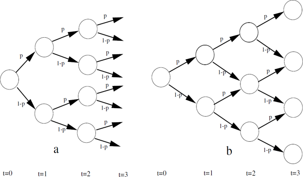
Two binomial trees — the one to the right is a so-called recombinant tree, where a given node can have two predecessors.
Before we go into details with the mathematical technicalities, we provide an example to guide the intuition.
Example 3.2 (Two period model).
Consider a two period model consisting of a riskless security, with initial value 1 and a deterministic interest rate r, and a stock with uncertain values at time t = 1,2. The uncertainty of the stock is modelled as a binomial tree, consisting of a binomial branch at the initial node at time t = 0, and binomial branches at the two possible nodes at time t = 1. By truncating the tree in Figure 3.2 at time t = 2, the evolution of the value of the riskless security and the stock price is given in Figure 3.3.

The initial value of the stock is assumed to be S. At time t = 1 we know whether the state of the world is either (ω1 or ω2) or (ω3 or ω4). If the state of the world is (ω1 or ω2) the value of the stock is uS, and the value is dS if the state is (ω3 or ω4). The value of the money market account is (1 + r) independent of the state of the world. At time t = 2 the state is known, and the value of the stock is listed in Figure 3.3. The value of the money market account is (1 + r)2.
Now suppose we want to price a European call option on the stock with exercise price K. The value of the option at time t = 2 is V = max(S_2(ω) − K, 0), where ω indicates that the stock price depends on the state of the world.
In the one-period model the arbitrage-free price is found by the value of a replicating portfolio (with the same cash flow at the end of the period). This principle will be applied in a recursive manner to the two period binomial model. We begin with the upper binomial branch at time t = 1. Let Cuu denote the value of the call option in state ω1 and Cdu in state ω2. As in the one-period model we want to determine a portfolio (ϕu, ψu) in the stock and the money market account, which replicates the value of the option at time t = 2. This is obtained by solving the linear system
ϕuu2S+ψu(1+r)2=Cuu,(3.27)ϕuduS+ψu(1+r)2=Cdu.(3.28)
The solution is,
ϕu=Cuu−CduuS(u−d),ψu=uCdu−dCuu(1+r)2(u−d).(3.29)
The value Cu of this portfolio is
Cu=ϕuuS+ψu(1+r)=11+r((1+r)−du−dCuu+u−(1+r)u−dCdu),(3.30)
and this is what the call is worth at time t = 1 if the first move was up. If the first move was down the value of the call Cd at time t = 1 can be determined in a similar way, thus
Cd=11+r((1+r)−du−dCud+u−(1+r)u−dCdd),(3.31)
where Cdd and Cud denote the value of the call at state ω4 and ω3 at time t = 2. Now we know what the call is worth at time t = 1 depending on which state we are in at that time. Looking at time t = 0 we want to construct a portfolio which gives us Cu if we are in state (ω1 or ω2) at time t = 1 and Cd is the state in (ω3 or ω4). Again we have a one-period problem, which we can easily solve, and the value of the replicating portfolio, which is equal to the value of the call C0 at time t = 0, is given by
C0=11+r((1+r)−du−dCu+u−(1+r)u−dCd).(3.32)
By inserting (3.30) and (3.31) in (3.32), and defining q=(1+r)−du−d, we get
C0=1(1+r)2(q2Cuu+2q(1−q)Cud+(1−q)2Cdd).(3.33)
We recognize that this expression shows that the value of a call option is found as the discounted value of the expected value of the payoff of the option at time t = 2, where the expectation is taken with respect to the risk-neutral probabilities. The risk-neutral probabilities denote the probabilities under the equivalent martingale measure ℚ, which we will discuss later. Formally we have
C0=1(1+r)2Eℚ[Ct=2].(3.34)
The important thing to learn from this example is the following: Starting out with the amount C0, an investor is able to form a portfolio of the stock and the money market account which produces the payoffs Cu or Cd at time t = 1 depending on where the stock goes. Now without any additional cost, the investor can rearrange his portfolio at time t = 1, such that the payoff at time t = 2 will match that of the option. Therefore, at time t = 0 the price of the option must be C0.
3.3.1 σ-algebras and information sets
In this section we shall present a general formula for derivative pricing in multiperiod models. Some important concepts from probability theory, like σ-algebras, probability spaces, partitions, etc., will be used. If the reader is not familiar with these concepts please consult Appendix B for a brief overview.
Given a probability space (Ω,ℱ,ℙ) with a finite sample space Ω, and ℱ the σ-algebra of all subsets of Ω, assume that ℙ(ω) > 0 for all ω ∈ Ω (no elements in Ω have probability zero). Also assume that there are T + 1 dates, starting at date 0, ending at time T. In the general theory of multiperiods models it will be shown that the pricing of derivatives consists of a conditional expectation, where the conditioning argument is the “information set” up to the present time. It is therefore important to formalize the concept of information, which is done by introducing σ-algebras. However, to illustrate how information is revealed through time, we give an example.
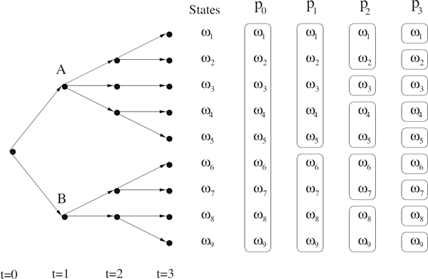
Example 3.3 (Event tree).
Consider the event tree in Figure 3.4 with three periods. In this example we shall only consider how we can represent knowledge in terms of partitions/σ-algebras, and not study a particular financial market. Suppose that an outcome ω ∈ Ω is chosen by “someone” or “something,” but the chosen state is unknown to us at time t = 0. We only know that one state has been chosen. This is represented by a partition ?0 containing one set, namely the entire sample space, which can be interpreted as no information. At time t = 1, we are in either state A or B, i.e., we know that the state is either (1) {ω1, ω2, ω3, ω4, ω5} or (2) {ω6, ω7, ω8, ω9}, which is formalized by the partition ℙ1 in Figure 3.4. At time t = 2 the partition is even richer. Thus, we know in which of the five subsets {ω1, ω2}, {ω3}, {ω4, ω5}, {ω6, ω7} or {ω8, ω9} the true state is. At time t = 3 we know exactly which of the states is the true state, and it is represented by a partition ℙ3 where each of the elements of ℙ3 contains one single state ωi cf. Figure 3.4. Thus as times goes by we obtain more information, and at time t = 3 we have complete information.
Although the “information set” from now on will be represented by σ-algebras, it is fruitful to think of it in terms of partitions and information sets that become more detailed as time goes by.
To formalize how information is revealed through time, we introduce the notion of a filtration.
Definition 3.3 (Filtration).
A filtration on (Ω, ℱ) is a family {ℱi}Ti=1 of σ-algebras in ℱ such that
ℱ0⊆ℱ1⊆...⊆ℱT.(3.35)
If ℱ0 = (Ø, Ω) and ℱT = ℱ the filtration may be considered as a sequence of information sets increasing from “no information” to “full information” — similar to the interpretation of partitions in Example 3.3.
Definition 3.4 (Adapted process).
A discrete time stochastic process (Xt)t=0,...,T is a sequence of stochastic variables X0, X1,..., XT. The process is said to be adapted to the filtration ℱ if Xs is ℱs-measurable, which is typically written as Xs ∈ ℱs.
3.3.2 Financial multiperiod markets
We are now ready to model financial markets as multiperiod models. Let St(ω)=(S0t,S1t,...,SNt) be a vector of adapted processes of the securities available on the market. This means that Sit(ω) is the price of security i at time t in state ω. Suppose one of the securities S0 is a money market account with initial value 1 and a deterministic interest rate r for all T periods. In the one-period model we defined a portfolio as an N-dimensional vector h, where hi denotes the number of security i bought at time t = 0. In a multiperiod model this concept ought to be generalized because the portfolio might change over time. Thus we obtain a portfolio vector at each time point. This is done in the following definition.
Definition 3.5 (Trading strategy).
A trading strategy is an (N)-dimensional vector of adapted processes
h=h1,h2,...hN(3.36)
with the interpretation similar to that of a one-period model, so denotes the number of security i held at time t in state ω.
The requirement that the trading strategy is adapted represents the very important idea that the strategy can only be based on the current level of knowledge. To illustrate this we assume we are in node A in Figure 3.4 at time t = 1. Then the trading strategy can base the number of securities on the fact that we are in node A and not in B. Notice that the number of securities may not be based on whether the true state is ω1, ω2, ω3, ω4 or ω5 (i.e., it is not allowed to base a trading strategy on information released in the future, for example, future values of the stocks). From an economical point of view, it clearly makes sense to require that the trading strategy should be an adapted process.
Definition 3.6 (Value process).
The value process at time t corresponding to h is defined as
Definition 3.7 (Self-financing trading strategy).
A trading strategy h is selffinancing if it satisfies
The interpretation of a self-financing strategy is that it is only allowed to change the portfolio in a way such that the total value of the portfolio does not change. However, the value of the trading strategy can of course change over time due to changes in the stocks. The definition of arbitrage in multiperiods models is based on the definition of self-financing portfolios.
Definition 3.8 (Arbitrage).
An arbitrage is a self-financing strategy for which
and
In words this definition says that there are arbitrage possibilities in the model if there exists a trading strategy with zero cost at the initial time with the following two properties: (1) No risk of getting any losses at the future time T; (2) A positive probability of getting a strictly positive payoff. If no arbitrage possibilities exist in the model, we say that the model is free of arbitrage. Compared with the definition of arbitrage in the one-period model (3.1) it is readily seen, that the above definition is a generalization.3
3.3.3 Martingale measures
The pricing of derivatives in discrete and continuous-time models is built on so-called martingale measures which basically are probability distributions that are related to the historical or objective probability distribution. In the one-period model we saw that the price of a derivative, e.g., an option, was given by the discounted value of the expected value of the payoffs at time t = 1, where the expectation was taken with respect to the so-called risk-neutral probabilities. In multiperiod models as well as continuous models, we basically use the same procedure for pricing derivatives.
Since the pricing formulas stated in the following rely on conditional expectations it is necessary to be familiar with this concept, in the case where the conditioning argument is a σ-algebra. In Appendix B a brief overview is given.
Definition 3.9 (Martingale).
A stochastic process X is a martingale with respect to the filtration if it satisfies
The best prediction is the current value
for all t = 1, 2, ..., T.
- Xt is adapted to the filtration ℱt for all t.
- The process has finite expectation
Remark 3.4.
In applications we shall mainly be interested in the first property in Definition 3.9, and just assume that properties 2 and 3 are fulfilled.
Let us consider two simple examples of martingales.
Example 3.4.
Consider a collection of independent and identically distributed stochastic variables X1,X2,... with mean zero E[Xi] = 0. Let ℱn = σ{X1,X2,...,Xn} denote the σ-algebra generated by X1,X2, ..., Xn. Furthermore, we introduce the filtration .
We wish to show that the sum
is an ?-martingale. From the linearity of the expectation operator, we get
The latter Sn−1 is ℱn−1-measurable, and the former has expectation zero. Hence
which shows that Sn is an -martingale.
Example 3.5.
We consider the same setup as above with the exception that E[Xi] = 1 and Xi > 0 for i = 1,2,....
We wish to show that the product
is a -martingale. Thus we must show that
As X1 · X2 ·...· Xn−1 is ℱn−1-measurable, we get
where the last equality sign follows from E[Xn] = 1.
Definition 3.10 (Equivalent measures).
Two probability measures ℙ and ℚ are said to be equivalent if they assign zero probability to the same sets A in the σ-algebra
Definition 3.11 (Equivalent martingale measure).
An equivalent martingale measure for the security market model S, defined on , is a probability measure ℚ on Ω with ℚ(ω) > 0 for all ω ∈ Ω such that each component in the vector ofdiscounted price processes
is a martingale, i.e.,
For the one-period model it was stated in Theorem 3.1 that a financial model is free of arbitrage if and only if there exists a state price vector. Using the concept of martingale measures we can state a similar, but more general, theorem.
Theorem 3.2.
In a discrete time security market with finite sample space the following two statements are equivalent.
- There are no arbitrage opportunities.
- There exists an equivalent martingale measure.
Proof. See Lando [1996].
Remark 3.5.
In Example 3.2 we found that the pricing formula for the call option was given by
which exactly shows that ℚ = (q2,2q(1 − q), (1 − q)2) is an equivalent martingale measure since
- Strictly positive probabilities are assigned to the three final states.
-
The stochastic process has the martingale property under the probability measure ℚ,
This leads us to the following theorem which is extremely useful for pricing various types of derivatives.
Theorem 3.3.
Let a security model S = (S 0,...,SN) be defined on , where S 0 is a risk-free asset, and assume that S is arbitrage-free and complete. Let ℚ denote the unique martingale measure for S. An extended model consisting of S and a new security price process C is free of arbitrage if and only if
Proof. See Musiela and Rutkowski [1997].
In the case where the discount rate is deterministic and constant, , the expression simplifies somewhat.
This arbitrage-free pricing formula can be applied to price options of various types, e.g., European call and put options, American options, etc. In the problems some of these are considered.
3.4 Notes
If the reader is further interested in the theory of discrete time finance Lando [1996] gives a excellent introduction and has some of the proofs that we have omitted, and a lot more. There are in Duffie [1996] a few chapters on discrete time finance which goes even further into the theory. This book is highly recommended, though it is written in a compact way.
3.5 Problems
Problem 3.1.
Consider a one-period model with two states (M = 2) and the following three securities:
- A stock with initial price and payoff D11 = GS0 in state 1 and payoff D12 = BS0 in state 2, where G > B > 0.
- A riskless bond with initial price and payoff D21 = D22 = (1 + r), where (1 + r) is the riskless return and (1 + r)−1 is the discounting factor.
- A call option on the stock, with initial price = C and payoffs D3j = max[D1j − K, 0] for both states, where K ≥ 0 is the exercise price of the option. (The call option gives its holder the right, but not the obligation, to pay K for the stock, after the state is revealed.)
- 1. Show necessary and sufficient conditions on G, B and (1 + r) for the absence of arbitrage involving only the stock and the bond.
- 2. Assuming no arbitrage for the three securities, calculate the call-option price C explicitly in terms of , G, (1 + r), B and K. Find the risk-neutral probabilities and in terms of G, B and R, and show that , where denotes the expectation with respect to
Problem 3.2.
Suppose we have a trinomial market free of arbitrage as described in Example 3.1. We have seen that this model is not complete since there are more states than traded asset. Now assume that a European call option with the value at time t = 1 is added to the market.
- 1. Determine the values of Kc, which completes the market consisting of the bond, the stock and the European call option.
- 2. Now assume that the market is complete. Determine the price of a European put option with the value at time time t = 1, in terms of the bond, the stock and the call option.
Problem 3.3.
A stock index is a weighted sum over some of the most important stocks traded on a particular market. The C20-index is an example on the Danish stock market which includes the 20 most traded stocks.
where . Now assume we have a two period model with 20 states and with the 20 most traded assets, and that the market is complete and free of arbitrage. Assume that the following is known at time t = 0: the weights wi, the initial prices of stocks S0, the payoff matrix D and a vector v indicating the number of stocks vi that are currently on the market.
1. Determine the value of a future contract which gives the exact value of the C20-index at time t = 1.
Now assume that the weights are unknown at time t = 0, but determined at time t = 1 as the fraction of the total market value that at time t = 1 is placed in stock i.
Problem 3.4.
Consider a one-period model of a financial market with two securities: a stock and a money market account with initial value B0 and a constant interest rate r = 6%. Let denote the value of the stock in state i(i = 1,2) at time t(t = 0,1).
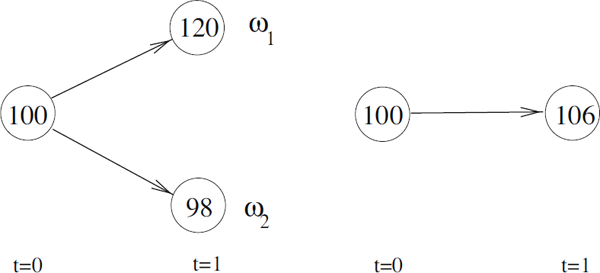
We wish to replicate a contract that pays 115 in state 1 and 95 in state
- 1. Determine the replicating portfolio (ϕ, ψ), i.e., a portfolio that contains ϕ units of the stock and ψ units of the bond.
- 2. Compute the fair price of the replicating portfolio at time 0.
-
3. Define the relative portfolio and fill out the table
r
2%
4%
6%
8%
10%
ϕ
ψ
ψ′
V
Comment on the results.
Problem 3.5
Consider a two period model of a financial model with a stock and a money market account with the constant interest rate r = 8%. Referring to Figure 3.3, the initial stock price is S = 100, S(ω1) = 121 and S(ω4) = 90.25. The probability of an increasing stock price is p = 0.70 and 1 − p = 0.30.
-
1. Determine the price in states 2 and 3. Is the event tree recombinant?
Now we wish to determine the arbitrage-free price of a European call option C0 with strike price K = 100, i.e., the payoff function is V = max(S2 − 100,0) = (S2 − 100)+, by constructing a replicating portfolio.
- 2. Assuming that the first stock price movement was upwards, determine the optimal portfolio.
- 3. Assuming that the first stock price movement was downwards, determine the value of the portfolio.
-
4. Compute the value of the replicating portfolio at time t = 0.
The following questions concern sensitivity analysis, i.e., an analysis of the changes in C0 due to variations in K and r.
- 5. Repeat the previous question for the strike prices K = 98 and K = 102.
- Compute the arbitrage-free price of the replicating portfolio for r = 6% and r = 10%. You may assume that K = 100.
1Although still very simple.
2This follows from Remark 3.2.
3In the one-period model two definitions of arbitrage were stated, where the first definition is directly comparable with the multiperiod definition of arbitrage.