Chapter 1
Introduction
In Théorie de la Speculation (1900), Louis Bachelier made the first attempt to model the inherent randomness in stock prices using a continuous-time counterpart of white noise, the Brownian Motion. For many years this modelling approach was of purely academic interest as financial institutions used less mathematically demanding methods. More than 70 years later the ideas proposed by Bachelier were used in two seminal papers by Robert Merton on continuous-time finance in general and Fischer Black and Myron Scholes on the pricing of options and corporate liabilities. Contrary to their own expectations, this area has expanded enormously during the last decades, and Merton and Scholes received the Nobel Prize in economics in 1997 for their research (Black passed away in 1995). The amount of money involved today is reported in Table 1.1, which can be compared to the US GDP which was about 15000 billion US dollar (USD) in 2012.
Notional and market value of outstanding OTC contracts in billions in US dollars December 2012. Data from Bank for International Settlements.
Contracts |
Notional value |
Market value |
Foreign exchange |
67358 |
2304 |
Interest rate |
489703 |
18833 |
Equity-linked |
6251 |
605 |
Commodity |
2587 |
358 |
Credit default swaps |
25069 |
848 |
Companies use these new products to protect themselves against changes in interest rates, foreign exchange rates and commodities prices. Mutual funds and pension funds use them to protect their stocks and bond investments. Major banks, brokerage firms and insurance companies write them for customers, while inventing such exotic names as caps, collars and swaptions.
The complexity of the vast range of new financial products that are continuously being introduced on the financial markets and the inherent uncertainty associated with stock prices, interest rates and foreign exchange rates have given rise to the emergence of a new scientific field: mathematical finance. This area of research encompasses the theory of stochastic processes (stochastic differential equations), partial differential equations, functional analysis and, last but not least, economics and finance.
In contrast to many other books on mathematical finance, this course will also cover the modern theory of financial derivatives from an empirical point of view. Thus identification and estimation theory play an integral part of the course. The reader should be able to utilize these methods in combination with methods in operations research for risk assessment, risk management and optimal portfolio selection. This combination of mathematical finance, statistics and operations research form the foundation of the science of financial engineering.
The ambitious and broad scope of the book can only be obtained at the expense of depth of coverage, so proofs and mathematical considerations of purely technical interest will be omitted for brevity. Nevertheless, it is our aim to bring the reader up to a level of understanding and managing empirical research in this area.
1.1 Introduction to financial derivatives
Let us introduce the merits of one of the most important financial derivatives, the European call option, by considering a fairly simple transaction between two companies. Assume that the Danish company IDEA A/S today (t = 0) orders 1 000 pieces of furniture from the American company Bench Inc. to be delivered in exactly 6 months' time (t = T). They have agreed upon a price of 500 000 USD, which should be paid upon delivery. We assume that the exchange rate today is 6 DKK/USD.
Due to the 6 months between the order and delivery date, IDEA A/S faces a serious risk regarding changes in the exchange rate between DKK and USD. Today (t = 0) they are unable to determine the exchange rate upon delivery (t = T) and hence the amount in DKK they are going to pay upon delivery is random. In the very unlikely case that the exchange rate should remain the same, they should pay 3 000 000 DKK, but if the exchange rate should go up to, say, 6.50 DKK/USD they will have to pay 3 250 000 DKK. From IDEA's point of view there is, of course, no problem associated with a possible lower exchange rate. Thus IDEA is exposed to an asymmetrical risk. There are at least three different ways of eliminating this risk.
I: The most naive approach would be to buy 500 000 USD today (t = 0) at the known exchange rate 6 DKK/USD, which would enable IDEA to avoid exposing themselves to a higher exchange rate at time t = T. This approach eliminates the risk, but there are a couple of noticeable drawbacks. First of all, a large amount of capital is tied up during the next 6 months, which might be put to more profitable uses. Second, they have lost the opportunity to take advantage of a lower exchange rate at time t = T.
II: A slightly more sophisticated approach would be to negotiate a forward contract with a participant on the foreign exchange (FX) markets that enables IDEA to buy 500 000 USD at time t = T at an exchange rate K determined at time t = 0. The exchange rate K (unit DKK/USD) is called the strike price and it is clearly specified in the contract.
No transactions are made at t = 0 and the amount to be paid at time t = T is fixed at K × 500 000 DKK. As the writer of the contract is obliged to sell the predetermined amount of USD at the predetermined strike price at time t = T, no matter what the exchange rate will be, this contract represents a value, and it is possible to trade it as any commodity for 0 < t ≤ T.
Let us say that a contract with a strike price of K = 6.2 DKK/USD has been negotiated, and that IDEA is obliged to pay 3 100 000 DKK in 6 months' time to the writer of the contract. If the exchange rate ST at time t = T is 6.5 DKK/USD, IDEA may congratulate themselves by having (indirectly) earned 150 000 DKK, because they would have been forced to pay 3 250 000 DKK if they had not written the contract. On the other hand, should the exchange rate drop to, say, 5.9 DKK/USD, they lose 150 000 DKK.
Again, IDEA has eliminated the risk of a higher exchange rate, but they are still unable to take advantage of a lower exchange rate.
III: Thus the question remains: Is it possible to write a contract that allows the holder of the contract (IDEA) to eliminate the risk and at the same time take advantage of a possible lower exchange rate? The answer is yes, and such a contract is called a European call option.
Definition 1.1
(European call option). A European call option on the amount of Y USD with exercise date T and strike or exercise price K is a contract, signed at time t = 0, that
- gives the holder of the contract the right to buy an amount Y dollars at the exchange rate K [DKK/USD] at time t = T, and
- allows the holder of the contract not to buy any dollars if the holder of the contract does not want to.
Options of this type (and a number of variations hereof) are traded on the international financial markets and the underlying asset can be anything from exchange rates to stocks, apples or oranges.
Note that purchasing an option on, say, an AP Møller stock is not the same as buying an AP Møller stock. The AP Møller stock is just the underlying asset that the holder has the right to buy if he finds it favourable.
Returning to IDEA, it now follows that they may buy a European call option on Y = 500 000 USD with exercise date T and strike price K = 6 DKK/USD. Should the exchange rate at time t = T exceed 6 DKK/USD, they may use (or exercise) the option and purchase the 500 000 USD at 6 DKK/USD from the writer of the contract. Conversely, should the exchange rate drop below 6 DKK/USD they can purchase the required amount of USD on the market and forget about the option.
Whereas the forward contract was, per definition, free, the option has a price. This price is determined by supply and demand on the option markets and it depends on the exercise date T and the strike price K. A higher strike price K gives rise to a lower price on the option, so IDEA is faced with the interesting problem of determining whether it is worth buying the option or not.
It is worth noting that this European call option is just one in an ever growing class of options that have at least two similarities:
- An option is a contingent claim which means that the holder of the option owns an uncertain claim on an underlying asset and that the value of the contract is contingent (conditional) on the future development of the price of the underlying asset.
- An option is a financial derivative as it exists solely in terms of the underlying asset and its value is derived from the (expected) value of this asset (in our case USD).
A major part of the course is to clarify what is meant by the fair, theoretical price of, e.g., a European call option and how to determine it. A brief overview of this project is as follows:
- We are considering a market with a number of given assets, such as stocks. The prices of these assets are assumed to vary randomly in time.
- We are going to introduce new financial products in terms of these given assets. These new products are called derivatives and typical examples are options, swaps, futures and forwards.
- We will then examine how to price such derivatives. The clue is that the derivatives are introduced in terms of already given assets with their own price processes and markets, so the derivatives cannot be priced at will. The complete market consisting of the given assets and the new derivatives must be priced consistently. In other words, the market should be efficient.
- It turns out that the valuation problem may be solved for a large number of derivatives such that each derivative is assigned a unique price. This price is called the arbitrage-free price of the financial derivative or financial instrument.
It is very important to remember that we are not going to determine the correct price, because the term “the correct price” of a derivative does not necessarily make any sense. We are just trying to determine the fair price in terms of the underlying assets.
Let us consider a very simple market where the uncertainty is limited to two different events in the sample space Ω = {ω1, ω2} with the probabilities P(ω1) = 0.8 and P(ω2) = 0.2. We are only considering the market at time t = 0 and t = 1 year. The market consists of two papers or so-called securities:
A bond with a deterministic price process given by
B0=100,B1=110.(1.1)
B0=100,B1=110.(1.1) This implies that the deterministic annual rate r is 10%. This can be seen by solving
B1=(1+r)B0(1.2)
B1=(1+r)B0(1.2) with respect to r. Note that the price of the bond (which could be a Danish Government bond) is used to determine the interest rate.
A stock with the price process S where S0 = 100 and S1 is given by
S1(ω)={125if ω=ω190if ω=ω2(1.3)
S1(ω)={12590if ω=ω1if ω=ω2(1.3)
That is the initial price of the stock is 100. At time t = 1 the price will be 125, if the outcome ω of our random process is ω1, or the price will be 90, if the outcome is ω2. In other words, we know the values of the assets at time t = 0, but the value of the stock depends on the outcome ω of the stochastic process.
We are now going to introduce a European call option with exercise date T = 1 and strike price K = 105 DKK in this simple market. This implies that the holder of the option has the right, but not the obligation, to buy a stock for 105 DKK. Assume that at t = 1, the random process generates the outcome ω1, then the value of the stock is 125 DKK and we exercise the option. Thus we have purchased a stock worth 125 DKK for 105 DDK and indirectly earned 20 DKK. Should the random process generate the outcome ω2, the value of the stock is 90 DKK, so we buy the stock at 90 DKK and forget about the option.
By purchasing the option we are faced with the stochastic income at time t = 1
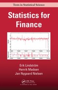
X=max [S1−K1,0]=max [S1−105].(1.4)
This is illustrated in the payoff diagram in Figure 1.1.
Payoff diagram for a European call option. For S < K, the option is not used. For S > K, the option is exercised and the amount S − K is (indirectly) earned.
The question is now how to determine the price Π(t,X) of the option at time t = 0. Two reasonable answers come to mind:
It seems reasonable to price the option such that the value of the option equals expected value of the future incomes (properly discounted)
∏(0,X)=βEℙ[X](1.5)
∏(0,X)=βEP[X](1.5) or equivalently
∏(0,X)B0=Eℙ[∏(1,X)B1](1.6)
∏(0,X)B0=EP[∏(1,X)B1](1.6) where the β = B0/B1 = 0.91 is the discount factor determined by the bond prices. It is important to note that the paper with the deterministic price process, i.e., a paper where the price is known with certainty at all times, is used to determine the present value of the payoff function X at time t = 1. We say that the future price (t = 1) of the option is discounted to determine the present value (t = 0) of this payoff. The discount factor β may be used to determine the so-called implied interest rate from the bond prices. We get the solution
∏(0,X)=β(ℙ(ω1)(125−105)+ℙ(ω2)⋅0)=0.91(0.8⋅20+0.2⋅0)=14.5 DKK.
In other words, the value of the option is expressed in terms of the bond prices. In this case, we say that the bond is chosen as the numeraire.
- From an economic point of view, it does not make any sense to talk about a correct price, because the price is determined by supply and demand on the market, and thus it depends on the perceptions of risk among the dealers on the market, which vary greatly among individuals as well as financial institutions.
As it will be shown later these answers are both right and wrong. Just to give the basic idea, the expected value in (1.5) should be taken with respect to another so called equivalent martingale measure ℚ than the objective probability measure ℙ in order to obtain arbitrage-free prices, and this martingale measure is determined uniquely in complete markets and in incomplete markets by the market participants (although they are probably not aware of it). Besides these technicalities, it is obvious that the price should depend on the uncertainty in the markets. This uncertainty is usually called the volatility and it is associated with the standard deviation of the interest rates, foreign exchange rates or stock prices, e.g., pension funds tend to invest their members payments in bonds which are less volatile than stocks.
1.2 Financial derivatives — what's the big deal?
A large number of these exotic derivatives were developed by quants (a Wall Street jargon for quantitative analysts) in the 1980s, where money was moving around the world as never before. This may partly be explained by historical events: the demise of communism in Eastern Europe that expanded markets for investors, the progression towards free enterprise in China, the liberalization of economic policies in Latin America and the rapid economic growth of the countries in the Far East.
Trespassing in such unchartered markets is a very risky business for western European and American companies. It is very difficult to assess whether a newly established company in an Eastern European country is able to pay the promised amount. The inflation, interest and foreign exchange rates may vary enormously and in a manner that is essentially unpredictable. Thus, the demand for security blankets or financial derivatives that were particularly designed to protect companies against these uncertainties was high. Before 1973 all such derivative contracts were traded as “over-the-counter” (OTC) products, i.e., a new derivative contract was individually negotiated by a broker on behalf of two clients, one being the buyer and the other the seller. Trading on an official exchange began in 1973 on the Chicago Board Options Exchange (CBOE) with trading initially only in call options on some of the most heavily traded stocks. Nowadays options are traded as “off-the-shelf” products on all of the world's major exchanges. They are no longer restricted to stock options but include options on indices, futures, government bonds, commodities, currencies, etc. The OTC market stills exists, and specific options are written by institutions to meet a client's needs. This is where exotic options, such as Parisian, Asian, Barrier and multi-asset options are created; they are very rarely quoted on an exchange.
The fundamental advantage of derivatives is that you can buy the risk that you want and eliminate (or hedge) the risk you do not want. Because there are two sides of each transaction, one party will pass along the risk he or she does not want to someone who wants to speculate. This also explains that derivatives can be both conservative and highly speculative investments. Hedging is used to spread the risk, but the implemented hedging strategies generate interlocking commitments of trillions of dollars in a kind of financial cyberspace. If something goes wrong, it might spread fast due to the use of modern computers, and the entire market may crash like a house of cards. This has happened several times during the last decade, the most famous event being the Flash Crash that occurred on May 6, 2010. The Dow Jones Industrial Average plunged almost 9% only to recover the losses within minutes when many market participants realized something was seriously wrong with the market. Still crashes of this type causes a lot of trouble; see Easley et al. [2011] for a discussion.
It's one of the inherent paradoxes of derivatives that the market volatility increases when each market participant aims at minimizing the volatility of his portfolio.
Beside these speculative applications of financial derivatives, they may be very valuable for more productive enterprises. The basic idea is that you can buy, e.g., an option on a stock that you would like to purchase at some future date (maybe you do not have the money today) for only a limited amount of money compared to the actual price of the stock; but you can choose not to buy it if the price is not right.
Let us just for the sake of argument disregard the fact that the usual expected value of future payments is not an appropriate mean of computing the price of a European call option.
Example 1.1 (Leverage).
Assume that an investor would like to purchase an AP Møller stock in six months' time. He or she writes an European call option on the stock with exercise date T (in six months) and exercise price 250p.1
If the AP Møller stock costs 270p at time T, then the investor would be able to purchase the stock for the exercise price 250p. Thus he has immediately made a profit of 20p, i.e., he or she can exercise the option and buy the stock at 250p and sell at the market value of 270p (assuming that there are no transaction costs associated with these trades). On the other hand, if the AP Møller stock is only worth 230p at time T, with equal probability, then the expected profit to be made is
12⋅0+12⋅20=10p
Ignoring interest rates for the moment, it seems reasonable that the order of magnitude for the value of the option is 10p.
Of course, valuing an option is not as simple as this, but let us suppose that the holder did indeed pay 10p for this option. Now if the stock price rises to 270p at expiry the investor has made a net profit of
profit on exercise |
= |
20p |
cost of option |
= |
−10p |
net profit |
= |
10p |
This net profit of 10p is 100% of the upfront premium (the price paid at t = 0). The downside of this speculation is that if the stock price is less than 250p at expiry, the investor has lost all of the 10p invested in the option, giving a loss of 100%. If the investor had instead purchased the stock for 250p at time t = 0, the corresponding profit or loss of 20p would have been only ±8% of the original investment. Option prices thus respond in an exaggerated way to changes in the underlying asset price. This effect is called leverage.
Thus the price of the option may grossly affect the expected profit, and the idea behind hedging is to fence off the risk and avoid paying the price of the option by option replication. That is, we construct a collection or a portfolio of papers (stocks, bonds and money accounts in the bank) such that we get the same payoff diagram of this portfolio as the one associated with the call option without actually buying the option. Option replication may also be used to construct a portfolio that is less volatile (risky) than the original portfolio. In other words, the option is essentially redundant, and this observation will be used for valuation, because the price of the option should be the same as the price of the replicating portfolio.
The moral is that financial derivatives should be used with caution, but there are obvious advantages associated with their use. Otherwise they probably would not exist!
This discussion should demonstrate that there a number of important questions of technical interest that need to be addressed:
- Identification: We need statistical methods to identify the structure of the models from time series data, mathematical concepts to analyze these models and the statistical tools to apply these models to observed data sets. One of the most important concepts is the volatility.
- Volatility: We need to assess the volatility, i.e., we need to model the stock prices, foreign exchange rates, etc. such that we can quantify the market and portfolio volatility using statistical estimation methods.
- Valuation: We need to define markets where existing and new derivatives may be priced consistently.
- Interest rates: It should be clear by now that the interest rate plays a fundamental role in determining the present value of future payments. Thus we need to estimate the interest rates at these future dates using the information that is available today. The bond market is used to express the market participants' expectations and the future interest rates are derived from the bond prices. Hence, the modelling of bond prices and interest rates are inherently important.
1.3 Stylized facts
Financial data have some pretty universal properties that differ from what we know about data in physics, biology or engineering.
There are several nice papers summarizing these stylized facts (Rydén et al. [1998], Cont [2001]). The most commonly mentioned are
- No Autocorrelation in returns
- Unconditional heavy tails
- Gain/Loss asymmetry
- Aggregational Gaussianity
- Volatility clustering
- Conditional heavy tails
- Significant autocorrelation for absolute value of the returns
- Leverage effects
We evaluate these claims on daily OMXS30 data from 1991–2014. The OMXS30 is an index composed of the 30 largest companies on the Swedish Stock market.
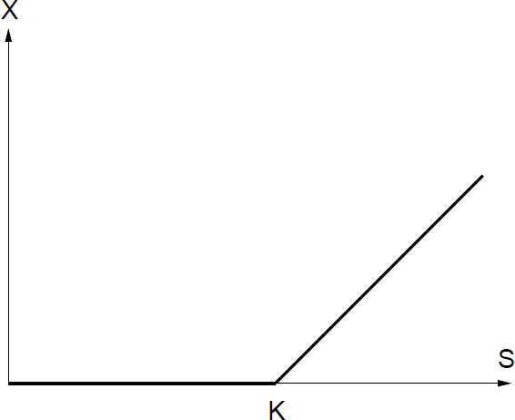
1.3.1 No autocorrelation in returns
There is very little (linear) autocorrelation in returns (Figure 1.2). This feature may not be surprising as investors being able to predict future values of assets would trade to benefit from the predictions. They would make a profit (on average) at the expense of their counterparties, who would then revise their forecasts or lose more money. The only long time surviving investors would be those who are able to predict well and revise their forecasts when new informations arrives.
Still some autocorrelation is often found in the first lags, due to trading friction, etc.
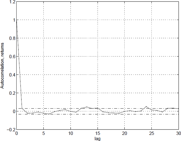
1.3.2 Unconditional heavy tails
The Gaussian distribution may be fine for many applications, but it does not represent the unconditional distribution of returns well. Large and extreme events are much more common than predicted by the normal distribution (Figure 1.3).
1.3.3 Gain/loss asymmetry
It is often claimed that losses are bigger in absolute value than gains (Figure 1.4). The losses (compared to the overall upward sloping trend) are bigger in amplitude and shorter in duration than the gains.
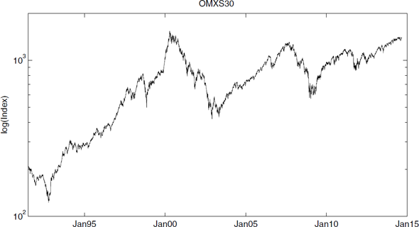
The evolution of the logarithm of OMXS30 between 1991 and 2014. Notice that losses are bigger and more rare than the gains.
This would be consistent with risk averse investors and the leverage effect discussed below.
1.3.4 Aggregational Gaussianity
Returns computed over long time periods are more Gaussian than returns computed for short time periods (Figure 1.5). The return over a long period can be written as a sum of returns over shorter periods. That suggests, under some conditions, that the return over long periods should become increasingly Gaussian.

Returns the OMXS30 computed using one week (r), two weeks (r2), four, eight, sixteen and thirty-two weeks of data.
This Central limit theorem type behavior indicates that the tails are heavy, but not as heavy as some early studies would indicate.
1.3.5 Volatility clustering
The volatility in linear Gaussian time series is constant, meaning that the variability is the same. This is not true for financial data, as we are experiencing calm periods and more volatile periods (Figure 1.6). Time varying volatility contributes to the heavy tails.
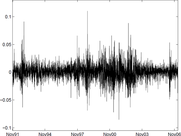
Modeling time varying volatility is an important topic, and is covered in Chapter 5.
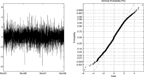
1.3.6 Conditional heavy tails
The returns are heavy-tailed, even when applying a model that compensates for the time varying volatility; cf. Figure 1.7. Events like earthquakes are extremely difficult to forecast, meaning that the volatility is going to be underestimated by virtually any volatility model during days when big unexpected events occur.
1.3.7 Significant autocorrelation for absolute returns
The volatility clustering clearly shows that returns {r(t)} are not independent and identically distributed, iid. Computing the autocorrelation for |r(t)| or r2 (t) reveals a different story (Figure 1.8). The effect can be found for power transformations of the absolute returns |r(t)|θ, θ > 0 but is most pronounced when θ = 1. This is known as the Taylor effect (e.g., Granger and Ding [1995]).
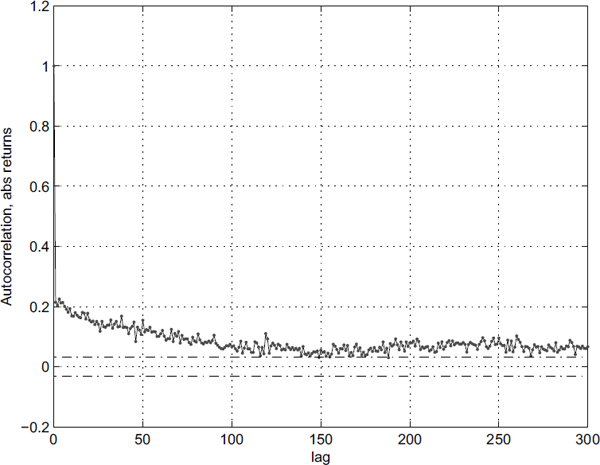
Sample autocorrelation for the absolute values of the returns, |r(t)|, showing significant dependence.
There is a significant dependence in the volatility (ranging for at least 150 days), perhaps even long range dependence. Recent studies, however (e.g., Nystrup et al. [2014]), indicate that this is probably not the case, but rather due to lack of stationarity. This would also explain why the dependence does not drop to zero at any point in the Figure.
1.3.8 Leverage effects
The leverage effects are really due to bookkeeping in firms. A company experiencing bad times will either take up additional debt or live off savings. The financial status will deteriorate in either case, resulting in additional uncertainty in future earnings. A decrease in stock price means that the company is more leveraged since the relative value of their debt rises with respect to their equity. The effect due to good news on the other hand is rarely of the same magnitude as that of bad news (Christie [1982], for a through discussion).
All of this results in a negative correlation between returns and the volatility, known as the leverage effect. Several models in Chapter 5 will take this stylized fact into account.
1.4 Overview
Now that we have established some of the fundamental terms in mathematical finance, we will sketch the contents of the remainder of this book.
Chapter 2, Fundamentals, will discuss applications of financial derivatives with respect to risk assessment and elimination. Some methods for computing the net present value of a future cash flow will be described using discount factors. Finally, continuously compounded interest rates, which provide the foundation of the remainder of the text, will be introduced.
Chapter 3, Discrete time finance, will introduce the concepts of arbitrage, probability measure transformations, self-financing portfolios and martingales in a simple financial market.
Chapter 4, Linear time series models, briefly reviews linear time series models and methods.
Chapter 5, Nonlinear time series models, extends the theory to nonlinear and/or nonstationary time series. An overview of a number of model classes is given. Emphasis will be placed on a description of the variance structure as the variance of, e.g., interest rates varies with time and depends on the current level of the interest rate. Such heteroscedastic behaviour cannot be described by linear models.
Chapter 6, Kernel estimators in time series analysis, describes some statistical methods for identification of discrete and continuous-time models of interest rates, foreign exchange rates, stock prices and other financial time series.
Chapter 7, Stochastic calculus, discusses the problem of introducing stochasticity in mathematical modelling of dynamical systems by means of the Wiener process. Focus is placed on Itō stochastic calculus.
Chapter 8, Stochastic differential equations, introduces stochastic differential equations (SDEs) and the important Itō formula is presented. The Feynman–Kac representation theorems establish a link between parabolic partial differential equations and SDEs, which may be used as a mean of computing prices of financial derivates and solving SDEs. Finally the Girsanov measure transformation is introduced. The concepts in this chapter may be used in many other areas of the natural and technical sciences.
Chapter 9, Continuous time security markets, provides a set of theoretical tools that makes it possible to determine the arbitrage-free price of the large variety of financial derivatives that are traded on the international markets. The celebrated Black & Scholes model is covered in detail, and a number of sensitivity parameters (the so called “Greeks”) are discussed.
Chapter 10, Stochastic interest rate models, uses the concepts of the previous chapter to describe a number of famous interest rate models.
Chapter 11, The term structure of interest rates, discusses the valuation of bonds. Bonds are essentially simple options, but they are tremendeously important for estimating the interest rate over a long period of time. This is called the term structure of interest rates and it provides the foundation for computing the present value of future payments.
Chapter 12, Discrete time approximations, provides sampling or discretization schemes for computing a discrete-time approximation of SDEs, which is required in the following chapters.
Chapter 13, Parameter estimation in discretely observed SDEs, introduces a very general maximum likelihood method for parameter estimation in continuous/discrete-time state space models. In addition the generalized method-of-moments (GMM) is discussed. The last method encompasses both the well-known method-of-moments and nonlinear least squares methods.
Chapter 14, Inference in Partially Observed Processes, provides a considerable extension of the estimation methods listed above which makes it possible to estimate parameters in multidimensional state space models (e.g., multifactor interest rate models). The Kalman filter is introduced for linear and nonlinear continuous-time models. The topics covered in this chapter are of general interest.
Appendix A, Projections in Hilbert spaces, provides a unified introduction to a number of filtering and estimation methods, which may geometrically be viewed as projections in Hilbert spaces.
Appendix B, Probability theory, covers the fundamentals of probability theory from a measure-theoretical point of view.
Each chapter is closed with a number of problems that should support and extend the material covered in the text. It is advised to solve as many problems as possible while reading the text. Some problems in the early chapters require very little mathematical skill and are intended to develop your intuition for financial reasoning, which will be very important in later chapters, where the mathematical concepts are significantly more difficult.
1This is short for pence, but the choice of unit ($, DKK, etc.) is not important for the argument.