Chapter 11

Term structure of interest rates

In this chapter the concept of no-arbitrage will be discussed in the interest rate markets, which we also refer to as the bond market. Just to motivate the discussion, it should be noted that trading in various types of bonds grossly exceeds trading in the financial derivatives considered so far.

In Chapter 3, we considered pricing in complete (and incomplete) markets in discrete time and showed that the existence of a state price vector resulted in an arbitrage-free market. In Chapter 9, we presented a similar theory in continuous time and the tremendously important result was the correspondence between the existence and uniqueness of an equivalent martingale measure and arbitrage-free prices.

In the Black & Scholes model it is possible to determine the arbitragefree price of a large class of financial derivatives. This result stems from the fact that it was possible to trade in the underlying asset (the stock) and thus generate replicating portfolios. However, this important result does not hold in the interest rate (or bond) markets as it is not possible to trade directly in the underlying asset, namely the interest rate itself. Nevertheless, a large number of interest rate derivative products exist as discussed in Section 2.4.

It could be said that the concept of arbitrage in the Black—Scholes model was based on a vertical argument across the underlying asset and the financial derivative. In the bond markets, the concept of arbitrage is considered horizontally through time.

In Chapter 2, we considered deterministic interest rates and introduced the money market account in Definition 2.2 for continuously compounded interest rates. In Chapters 7—8, we introduced stochastic calculus and stochastic differential equations. These techniques were used in Chapter 9 to determine the arbitrage-free price of any financial derivative under the basic assumption that the interest rate was deterministic.

The objective of this chapter is to extend the theory to cover stochastic interest rates. In particular, we wish to discuss various types of interest rates such that we may determine the discounting factor in, e.g., (9.75) for stochastic interest rates. Basically, we wish to answer the following questions:

• Q1: How can one determine the interest rate at a future date when it is stochastic, i.e., described by a stochastic differential equation?
• Q2: How can one discount future payments (i.e., the payoff of a financial derivative) when the discounting factor is stochastic?

This chapter is organized as follows: Section 11.1 introduces a number of important concepts. Section 11.2 derives the term structure of interest rates using the classical approach. In Section 11.3 specific models of the term structure of interest rates are considered based on the interest rate models from Chapter 10. Section 11.4 briefly considers the socalled Heath—Jarrow—Morton framework for modelling the forward rates. As usual the chapter concludes with some notes and problems.

It should be stressed that this exposition does neither go into institutional details nor into the finer differences between the wide range of fixed income securities such as corporate bonds, mortgage backed securities and collateralized mortgage obligations (CMO). Some references will be given in the Notes.

11.1 Basic concepts

A bond is a contract, paid for up-front, that yields a known amount on a known date in the future, called the maturity date, t = T. The main purpose of a bond issue is to raise capital, and the up-front premium can be considered as a loan to the government or the company. In Denmark, bonds are issued by the government (i.e., The National Bank), all the major banks and a few trade-specific mutual funds.

A cash flow may be associated with the bond such that a cash dividend (or coupon) is paid out to the holder of the contract at fixed times during the lifetime of the contract. If there are no coupons the bond is known as a zerocoupon bond or just a zero-bond.

Definition 11.1 (A zero-coupon bond).

A (zero-coupon) bond with maturity date T is a contract that gives the holder of the contract C units of account (e.g., DKK) at time T. The price at time t of a T-bond is denoted by P(t, T).

Example 11.1 (Zero-coupon bonds).

On the Danish market, there will typically be three zero-coupon bonds in circulation. These are called skatkammer-beviser and have been issued by the Ministry of Finance since 1st April 1990. They have a relatively short lifetime of 3, 6 and 9 months, and the face value C is 1 000 000 DKK. These zero-bonds are traded under circumstances that differ from other bonds, e.g., the price is determined through an auction.

11.1.1 Known interest rates

We now derive an equation for the value of the bond P(t, T) at time t prior to the maturity date T. We assume that the interest rate r(t) and the coupon payments K(t) are known functions of time. Thus we assume that cash coupon payments may also be made continuously in time. Such payments are often called dividends. The change in the value of one bond P(t, T) in the time interval [t, t + dt[is

$\frac{\text{d}P}{\text{d}t}\text{d}t.$

If we have received a coupon payment K(t) during the time period dt, our holdings (including the cash) change by the amount

$\left(\frac{\text{d}P}{\text{d}t}+K(t)\right)\text{d}t.$

Alternatively, we may also choose to deposit our capital in a savings account with the known interest rate r(t) and the value V(t). In order to exclude arbitrage possibilities, we must have

$\frac{\text{d}P}{\text{d}t}+K(t)=r(t)V(t)=r(t)P(t,T).(11.1)$

Otherwise a riskless profit may be made by moving our holdings from the savings account to the bond (>) or vice versa. With the final condition P(T, T) = C, this ordinary differential equation may be shown to have the solution

$P(t,T)=exp\left(-{\displaystyle \underset{t}{\overset{T}{\int }}}r(s)\text{d}s\right)\left(C+{\displaystyle \underset{t}{\overset{T}{\int }}}K(u)exp\left(-{\displaystyle \underset{t}{\overset{T}{\int }}}r(s)\text{d}s\right)\text{d}u\right).(11.2)$

Assuming that there are no coupon payments K(t) = 0, we get

$P(t,T)=Cexp\left(-{\displaystyle \underset{t}{\overset{T}{\int }}}r(s)\text{d}s\right)(11.3)$

from (11.2). If the bond prices P(t, T) are quoted today at time t for all values of the maturity date T, then we know the left-hand side of (11.3) for all T. Thus we may compute

$-{\displaystyle \underset{t}{\overset{T}{\int }}}r(s)\text{d}s=log[P(t,T)],(11.4)$

where we have assumed that C = 1. This is a standard convention which states that the bond pays out 1 unit of account at time T. This unit of account may be 1 000 DKK (e.g., skatkammerbeviser) or some other appropriate value. It is merely a question of choosing a normalizing factor such that the mathematical computations may be slightly simplified, i.e., we may exclude the log C term because log 1 = 0.

Assuming that P(t, T) is differentiable with respect to T, we get

$r(T)=-\frac{1}{P(t,T)}\frac{\partial P}{\partial T}(t,T).(11.5)$

Thus assuming that the prices of zero-coupon bonds genuinely reflect a known interest rate we may compute that interest rate at future dates T > t from the bond prices.

Since interest rates r(t) are inherently positive, we must have

$\frac{\partial P}{\partial T}(t,T)<0(11.6)$

which shows that the longer a bond has to live, the less it is now worth. In other words, the longer you have to wait to get the payment of C DKK the less this amount is worth to you today.

11.1.2 Discrete dividends

So far we have assumed that coupon payments were made continuously in time. However, in practice, coupon payments are only made at discrete time instants t = (t1,...,tN)′, i.e., every three, six or twelve months or so. With respect to (11.1) this may be modelled using the Dirac delta “function”

$\frac{\partial P}{\partial T}+K_c\delta (t-t_c)=r(t)V(t)=r(t)P(t,T)(11.7)$

where we have assumed that only one coupon payment Kc is made at time tc for simplicity. The solution is

$P(t,T)=exp\left(-{\displaystyle \underset{t}{\overset{T}{\int }}}r(s)\text{d}s\right)\left(C+K_c\mathscr{H}(t_c-t)exp\left(-{\displaystyle \underset{t}{\overset{T}{\int }}}r(s)\text{d}s\right)\right)(11.8)$

where the Heaviside function is given by

$\mathscr{H}(x)=\underset{-\infty }{\overset{x}{\int }}\delta (s)\text{d}s=\{\begin{array}{cc}0& \text{for}x<0\\ 1& \text{for}x\ge 0\end{array}$

or in other words

${\mathscr{H}}^{\prime }(x)=\delta (x).$

Let us consider the effect of a discrete coupon payment Kc at time tc on the price of the coupon bond. Prior to time tc, the bond has the value $P(t_c^{-},T)$ and immediately after, at time $t_c^{+}$, the value of the coupon bond is decreased by the coupon payment Kc:

$P(t_c^{+},T)=P(t_c^{-},T)-K_c.(11.9)$

This will be called the jump condition, and it will still apply when we move on to consider stochastic interest rates. The coupon payment also implies that the bond price is not continuous. In turn this implies that the derivation of (11.5) is not valid. The jump condition is illustrated in Figure 11.1 for real market data.

Remark 11.1 (Notation).

As the maturity date T is a parameter, we occasionally use the notation

$P^T(t)=P(t,T).$

Clearly we have

$P^t(t)=P(t,t)=1,\mathrm{for}\mathrm{all}t\ge 0(11.10)$

which states the price of a bond at time t that matures at time t is 1.

11.1.3 Yield curve

If we consider stochastic interest rates, P(t, T) becomes a stochastic process for every fixed T. Thus as a function of the time parameter t the trajectories of P(t, T) become highly irregular (Figure 11.1). For a fixed t (and a fixed trajectory ω) the price process P(t, T) is typically a smooth function and in particular differentiable with respect to T. Thus we introduce the notation

$P_T(t,T)=\frac{\partial P(t,T)}{\partial T}.$

The objective is now to determine the price process P(t, T).

Definition 11.2 (Forward rates).

For t ≤ S ≤ T the forward rate for the time period [S, T] at time t is defined as

$R(t,S,T)=-\frac{log[P(t,T)]-log[P(t,S)]}{T-S}.(11.11)$

The instantaneous forward rate at time T seen from time t is defined as

$f(t,T)={\displaystyle \underset{S\to T}{lim}}R(t,S,T)=-\frac{\partial log[P(t,T)]}{\partial T}.(11.12)$

We consider a special case of (11.11) in the following definition.

Definition 11.3 (The yield curve).

The forward rate for the period [t, T] is defined as

$Y(t,T)=R(t,t,T)=-\frac{log[P(t,T)]}{T-t}.(11.13)$

A plot of Y (t, T) against T −t is called the yield curve.

In the following definition, we introduce the most important concept in this chapter, namely the term structure of interest rates.

Definition 11.4 (The term structure of interest rates).

The dependence of the yield curve on the time to maturity T − t is called the term structure of interest rates.

Remark 11.2.

The terms “the yield curve,” “the term structure of interest rates” and bond prices are used interchangeably in the financial literature due to the following relationship.

From (11.13), we immediately get

$P(t,T)=exp[-Y(t,T)(T-t)](11.14)$

which shows that Y(t, T) is the implied average interest rate for the time period [t, T]. The yield curve is another measure of future values of interest rates than (11.5). The yield curve has a couple of advantages which are important for empirical work, namely

• The bond prices P(t, T) need not be differentiable, and
• a continuous distribution of bonds with all maturities is not required.

Example 11.2 (The yield curve).

Consider three zero-coupon bonds (skatkam-merbeviser (SKBV)) with maturities T1 < T2 < T3 and a face value C of DKK 1 000 000. From (11.14), it follows that

$\begin{array}{cc}P(t,T_1)=exp\left(-{\displaystyle \underset{t}{\overset{T_1}{\int }}}r(s)\text{d}s\right)=exp(-R_1(T_1-t))& (11.15)\\ P(t,T_2)=exp\left(-{\displaystyle \underset{t}{\overset{T_2}{\int }}}r(s)\text{d}s\right)=exp(-R_2(T_2-t))& (11.16)\\ P(t,T_3)=exp\left(-{\displaystyle \underset{t}{\overset{T_3}{\int }}}r(s)\text{d}s\right)=exp(-R_3(T_3-t))& (11.17)\end{array}$

where the yield is denoted by Ri, i = 1,2,3, after the continuous convention used in Denmark.

In practice the yield is the interesting quantity when discussing zerocoupon bonds rather than the integral over continuously compounded interest rates as the latter cannot be observed in the market. A selection of real prices and yields is presented in Table 11.1.

An interesting and important observation from Table 11.1 is that the yield is not constant. The yield varies with the maturity of the bonds. This should come as no surprise, since this is exactly the same situation as in the bank where a savings account pays a higher interest than a check account. In other words, the longer your investment horizon the higher the return. This observation, that the interest rate depends on the investment horizon, is expressed by the zero-coupon term structure ofinterest rates (or, in short, the term structure). It is clear that only a limited number ofpoints on the term structure is available, and our problem is basically to determine a reasonable interpolation method. We also note that the prices and the maturities confirm (11.6), namely that the price and the yield move in adverse directions.

From empirical market data it is observed that yield curves typically come in three distinct shapes (as illustrated in Figure 11.2), each associated with different economic conditions:

• Increasing: this is the most common form for the yield curve as it shows that future interest rates are higher than the short interest rate, since it should be more rewarding to tie money up for a long time than for a short time. E.g., the interest rate of a savings account is typically larger than for a check account.
• decreasing: this is typical of periods when the short rate is high but expected to fall.
• humped: again the short rate is expected to fall, although in a more complicated manner.

Now the last type of interest rates to be considered in these notes is defined.

Definition 11.5 (The spot interest rate).

The instantaneous (spot) interest rate at time t is defined by

$r(t)=f(t,t)(11.18)$

where f (t, t) is given by (11.12).

Note that the spot interest rate (for which a number of SDE models were proposed in Chapter 10) is connected to the forward rate. The spot interest rate r(t) is simply the forward rate obtained by investing our money in a bond in the time interval [t, t + dt]. For obvious reasons the spot rate is also called the instantaneous rate of interest or the short rate. The process of continuously investing our holdings at the spot rate r(t) is referred to as rolling over the money (see the discussion later on page 220).

All of the considered interest rate concepts are illustrated in Figure 11.3.

11.1.4 Stochastic interest rates

In the following we assume that the spot rate, the bond price and the forward rate may be described by the univariate Itō SDEs

$\begin{array}{cccc}\hfill \text{d}r(t)& =& \mu (t)\text{d}t+\sigma (t)\text{d}W(t)\hfill & \hfill (11.19)\\ \hfill \text{d}P(t,T)& =& m(t,T)P(t,T)\text{d}t+\nu (t,T)P(t,T)\text{d}W(t)\hfill & (11.20)\\ \hfill \text{d}f(t,T)& =& \alpha (t,T)\text{d}t+\sigma (t,T)\text{d}W(t)\hfill & (11.21)\end{array}$

where W(t) is a standard Wiener process defined on the usual filtered probability space (Ω, ℱ, ℙ).

The functions μ(t) and σ(t) may depend on r(t), while m(t, T) and ν(t, T) may depend on P(t, T) and so forth; we use this slightly more sloppy notation for convenience. The functions μ and σ are adapted processes, defined for all t ≥ 0. For every fixed T, the functions m(·, T), ν(·, T), α(·, T) and σ(·, T) are adapted processes defined for 0 ≤ t ≤ T.

Assumption 11.1.

In situations where some of the SDEs (11.19)—(11.21) are given, we assume that the involved processes are continuous functions oft and twice differentiable continuous functions of the parameter T. Furthermore we assume that

$\nu (T,T)=0,forallT\ge 0.(11.22)$

Remark 11.3.

The assumption (11.22) is a necessary condition for (11.20) to satisfy the boundary condition (11.10). It may be shown that this boundary condition also implies that the drift term m(t, T)P(t, T) in (11.20) should be finite with probability 1.

From the definitions of the bond prices, spot rates and forward rates, it is clear that the infinitesimal characteristics in (11.19)—(11.21) are related to one another.

Lemma 11.1

(From P(t, T) to f(t, T)). Let P(t, T) for every fixed T be described by (11.20). Then f(t, T) for every fixed T is described by (11.21) where

$\begin{array}{cc}\alpha (t,T)=\nu (t,T){\nu }_T(t,T)-m_T(T,T)\hfill & (11.23)\hfill \\ \sigma (t,T)=-{\nu }_T(t,T)\hfill & (11.24)\end{array}$

where vT(t, T) = ∂v/∂T(t, T), etc.

Proof. First, we write (11.20) in stochastic integral form

$P(t,T)=P(0,T)+{\displaystyle \underset{0}{\overset{t}{\int }}}m(s,T)P(s,T)\text{d}s+{\displaystyle \underset{0}{\overset{t}{\int }}}\nu (s,T)P(s,T)\text{d}W(s).(11.25)$

Taking derivatives with respect to T yields

$\begin{array}{c}{P}_T(t,T)=P_T(0,T)+{\displaystyle \underset{0}{\overset{t}{\int }}}\{m_T(s,T)P(s,T)+m(s,T)P_T(s,T)\}\text{d}s\hfill \\ +{\displaystyle \underset{0}{\overset{t}{\int }}}\{{\nu }_T(s,T)P(s,T)+\nu (s,T)P_T(s,T)\}\text{d}W(s)(11.26)\hfill \end{array}$

or in SDE form

$\begin{array}{c}d{P}_T(t,T)=\{m_T(t,T)P(t,T)+m(t,T)P_T(t,T)\}\text{d}t\hfill \\ +\{{\nu }_T(t,T)P(t,T)+\nu (t,T)P_T(t,T)\}\text{d}W(t).(11.27)\hfill \end{array}$

From (11.12), it follows that

$f(t,T)=-\frac{P_T(t,T)}{P(t,T)}=\phi (P_T(t,T),P(t,T))(11.28)$

where the function φ(·, ·) has been introduced.

In order to apply the multidimensional Itō formula (8.18) to this function, we need

$\begin{array}{l}\frac{\partial \phi }{\partial t}=0,\frac{\partial \phi }{\partial P}=\frac{P_T}{P^2},\frac{\partial \phi }{\partial P_T}=-\frac{1}{P},\frac{{\partial }^2\phi }{\partial P\partial P_T}=\frac{1}{P^2},\\ \frac{{\partial }^2\phi }{\partial P^2}=-2\frac{P_T}{P^3},\frac{{\partial }^2\phi }{\partial P_T^2}=0,\frac{{\partial }^2\phi }{\partial P_T\partial P}=\frac{1}{P^2}.\end{array}$

Now (8.18) yields

$\begin{array}{cc}\begin{array}{c}\text{d}\phi =0\cdot \text{d}t+\frac{P_T}{P^2}\text{d}P-\frac{1}{P}\text{d}{P}_T+\frac{1}{2}\frac{1}{P^2}\text{d}P\text{d}{P}_T+\frac{1}{2}(-2)\frac{P_T}{P^3}(\text{d}P{)}^2\hfill \\ +\frac{1}{2}\frac{1}{P^2}\text{d}{P}_T\text{d}P+\frac{1}{2}\cdot 0(\text{d}{P}_T{)}^2\hfill \end{array}\hfill & (11.29)\hfill \end{array}$

where the shorthand notation should be clear.

By inserting (11.20) for dP and (11.27) for dPT herein, we get, after some trivial computations,

$\begin{array}{cc}\begin{array}{c}\text{d}\phi =\left[m\frac{P_T}{P}-m_T-m\frac{P_T}{P}+\nu {\nu }^T+{\nu }^2\frac{P_T}{P}-{\nu }^2\frac{P_T}{P}-{\nu }^2\frac{P_T}{P}\right]\text{d}t\hfill \\ +\left[\nu \frac{P_T}{P}-{\nu }_t-\nu \frac{P_T}{P}\right]\text{d}W(t).\hfill \end{array}\hfill & (11.30)\end{array}$

Now the results in (11.23) readily follow.

The reader is encouraged to perform all the computations in this proof in detail. The results in Remark 8.6 on page 150 may be helpful.

Lemma 11.2

(From f(t, T) to r(t)). Assume that f(t, T) for every fixed T is described by the SDE in (11.21). Then r(t) may be described by (11.19) where

$\begin{array}{cccc}\mu (t)& =& f_T(0,T)+\alpha (t,t)+{\displaystyle \underset{0}{\overset{t}{\int }}}{\alpha }_T(s,t)\text{d}s+{\displaystyle \underset{0}{\overset{t}{\int }}}{\sigma }_T(s,t)\text{d}W(s)\hfill & (11.31)\\ \sigma (t)\hfill & =& \sigma (t,t).\hfill & (11.32)\end{array}$

Proof. This proof is omitted as it is of purely technical nature and quite hard. See Björk [2009].

Lemma 11.3

(From f(t, T) to P(t, T)). Let f(·, T) be described by (11.21) for every fixed T. Then P(t, T) may be described by the SDE

$\text{d}P(t,T)=(r(t)+b(t,T))P(t,T)\text{d}t+a(t,T)P(t,T)\text{d}W(t)(11.33)$

where the functions a(t, T) and b(t, T) are given by

$\begin{array}{cccc}a(t,T)& =& -{\displaystyle \underset{t}{\overset{T}{\int }}}\sigma (t,s)\text{d}s\hfill & (11.34)\\ b(t,T)& =& -{\displaystyle \underset{t}{\overset{T}{\int }}}\alpha (t,s)\text{d}s+\frac{1}{2}{a}^2(t,T).\hfill & (11.35)\end{array}$

In relation to (11.20), we have

$\begin{array}{cccc}m(t,T)& =& r(t)+b(t,T)\hfill & (11.36)\\ \nu (t,T)& =& a(t,T).\hfill & (11.37)\end{array}$

Proof. Omitted. See Björk [2009].

The forward rate R(t, S, T) is the return over the time period [S, T], t ≤ S ≤ T, of a bond purchased at time t, and f(t, T) is the instantaneous return at time T of a bond purchased at time t (see Figure 11.3).

From (11.18), we get that r(t) = f(t, t), which shows that we may interpret the spot rate r(t) as the instantaneous return of a bond with expiry t + dt purchased at time t. Thus the spot rate is the return of the following trading strategy: At every time instant t, we invest our entire wealth in a bond that is just about to mature. Such a strategy is called a roll-over strategy. Formally the value process V(t) of the roll-over strategy is

$\text{d}V(t)=V(t)u(t)\frac{\text{d}P(t,t)}{P(t,t)}$

where u(t) denotes the fraction of our wealth invested in the bond at time t. A roll-over strategy is thus defined by u(t) = 1 for all t. From (11.33), we get

$\frac{\text{d}P(t,T)}{P(t,T)}=\{r(t)+b(t,T)\}\text{d}t+a(t,T)\text{d}W(t).$

It follows immediately from (11.125) that a(t, t) = b(t, t) = 0 such that we get

$\text{d}V(t)=V(t)r(t)\text{d}t.(11.38)$

Thus the possibility of using a roll-over strategy on the bond markets implies the existence of a locally riskless paper with the stochastic interest rate r(t). Note that the paper is riskless although the interest rate is a stochastic process, because the interest rate process r(t) is adapted, which means that r(t) is known at time t (recall that the pricing formulas for financial derivatives are conditioned on ℱ(t)). To be precise, it should be said that future interest rates are stochastic.

So far we have considered the internal relations between bond prices and various types of interest rates. We have yet to determine the fair price of a bond.

Thus we wish to answer the following questions:

• Q3: Assume that the dynamics of the short rate r(t) is known. Which bond prices will be consistent with this particular choice ofr(t) and is it possible to determine unique bond prices from r(t) and the no-arbitrage requirement?
• Q4: Which restrictions must be imposed on P(t, T), 0 ≤ t ≤ T, in order to obtain an arbitrage-free money market?
• Q5: Which restrictions must be imposed on f(t, T), 0 ≤ t ≤ T, in order to obtain an arbitrage-free money market?
• Q6: What can we say about the prices offinancial derivatives in an arbitragefree money market? Is it, e.g., possible to determine the arbitrage-free price of a European call option on a bond?

11.2 Classical approach

Let us now model the short rate of interest r(t) by the univariate Itō stochastic differential equation

$\text{d}r(t)=\mu (t,r(t))\text{d}t+\sigma (t,r(t))\text{d}W(t)(11.39)$

where μ and σ are adapted processes, and W(t) is a standard Wiener process defined on the usual probability space (Ω, ℱ, ℙ).

The only possibility of investing our capital a priori is to invest it in the bank using a roll-over strategy. As argued above this implies that our capital evolves according to the ordinary differential equation

$\text{d}B(t)=r(t)B(t)\text{d}t.(11.40)$

We have considered this money market account repeatedly before, but we should now take into account that the interest rate is stochastic. As argued previously the possibility of using a roll-over strategy implies the existence of a paper with the price process given by (11.40). Now we formalize this as an assumption.

Assumption 11.2 (Price process B(t)).

On the capital market, there exists a financial security, B(t), with a price process given by (11.40), where the interest rate dynamics of r(t) is given by (11.39).

The value of a bond clearly depends on the (expected value of the) future evolution of the short rate of interest r(t), so we may consider a bond as an interest rate derivative.

Our primary interest is now to discuss what can be said about the structure of the prices of bonds P(t, T) with different maturity dates (Q3). We are faced with the difficulty that it is not possible to trade in the underlying asset, namely the interest rate.

Recall that the arbitrage-free price of a financial derivate in the Black-Scholes model was determined by Δ-hedging a portfolio consisting of a bond and a stock (the underlying asset). In particular, we could trade in both the bond and the stock, and thus generate a replicating portfolio. With respect to bond pricing, there is no underlying asset to trade in, thus we must make the arbitrage argument using at least two bonds with different maturity dates T1 and T2.

Before we formalize this approach, let us consider if we can expect to obtain a complete market and if we can determine unique, arbitrage-free prices in this market.

Let us for a moment consider a financial market with M securities (bonds, options, etc.) and N independent sources of noise (Wiener processes). For instance in the Black-Scholes model, we have M = 2 and N = 1 and we recall that this market is complete and arbitrage-free. We see that M = 2 and N = 1 satisfies the relation M = N + 1 and we may wonder if this relation is generic or if it is merely a coincidence. What happens if M ≤ N + 1 or M ≥ N + 1?

The first important observation is that the concepts of no-arbitrage and completeness introduce diametrically opposite restrictions on M versus N. If for instance we fix the number of random sources, N, then each new security yields arbitrage possibilities, which imply that the number of papers should be small compared to the number of random sources, which means that M ≤ N + 1. On the other hand, each new paper allows us to replicate a given financial derivative X using a replicating portfolio. Thus completeness requires a large number of securities compared to the number of random sources, i.e., at least M ≥ N + 1.

We state these results in a metatheorem, which does not have a precise mathematical meaning. In each particular case, we should rephrase the metatheorem as a genuine theorem.

Theorem 11.1 (No-arbitrage and completeness metatheorem).

Let M denote the number of a priori given securities (including the risk-free paper, if any). Let N denote the number of independent random sources. Then we have

• The market is arbitrage-free if and only if M ≤ N + 1.
• The market is complete if and only if M ≥ N + 1.
• The market if arbitrage-free and complete if and only if M = N + 1.

Proof. The proof is far from trivial in the general case (Delbaen and Schachermayer [1994, 1998] for details). However, the arguments presented above should make it plausible that this holds for diffusion processes.

Remark 11.4 (Geometrical interpretation).

Let M′ denote the number of securities excluding the riskless paper B(t), i.e., M′ = M − 1. Then we should have M′ = N in order to obtain an arbitrage-free and complete market. Interpret a realization of the N random sources at time t as a point in the N-dimensional Euclidean space. If M′ = N then we have a sufficient number of papers to reach this point (to eliminate the randomness, so to speak).

For the financial market described by (11.39) and (11.40), it follows that there is one security M = 1 and one random source N = 1. Thus the market is arbitrage-free, but it is not complete. Thus it should be expected that we cannot price a bond uniquely in terms of the riskless paper B(t). The number of securities is simply too limited to enable us to construct a replicating portfolio. However, this does not imply that the fair price of a bond can be an arbitrary value. On the contrary, the point is that in order to obtain arbitrage-free prices, bonds with different maturity dates must satisfy some internal consistency conditions.

In other words, if we assume that the fair price of one bond with a fixed maturity date T is given, then all other bonds may be priced uniquely in terms of this bond (and the short rate of interest).

This statement is in complete accordance with (Meta)theorem 11.1 because the market consists of the riskless paper B(t), the short rate of interest model and the bond yields N = 1 and M = 2. The particular bond given above is called the benchmark and it is very important to note that the price of all other bonds are given conditioned on the price of the benchmark bond. In practice, it is, by no means, a trivial task to determine the benchmark.

In order to make the arbitrage argument, we replace the previous assumption by the following.

Assumption 11.3.

Assume that there exists a financial market consisting of the riskless paper B(t) described by (11.40) and bonds for every choice of maturity date T ≥ 0. In addition, assume that the market is arbitrage-free and that the price of a T-bond may be written on the form

$P(t,T)=F(r(t),t,T)(11.41)$

where F is only a function of three real valued variables, and r(t) is given by (11.39).

As T is a parameter, we may also write FT (r, t) = F(r, t, T). It follows immediately from (11.10) that

$F(r,T,T)=1\text{for}\text{all}r.(11.42)$

Given this boundary condition, we will now determine the properties of the function F, see (Q4). In the following derivation, we write μ for μ(t, r(t)), and FT for F(r(t), t, T), etc., for simplicity.

In order to obtain portfolios consisting of bonds with different maturity dates, we need to determine the dynamics of each T-bond. By applying the Itō formula (8.10) to (11.41) and (11.39), we get

$\text{d}{F}^T=\left(F_t^T+\mu F_r^T+\frac{1}{2}{\sigma }^2{F}_{rr}^T\right)\text{d}t+\sigma F_r^T\text{d}W(t)(11.43)$

where $F_t^T=\partial F^T/\partial t$, etc.

By introducing the following in (11.43)

$\begin{array}{cccc}{\alpha }_T& =& \frac{F_t^T+\mu F_r^T+\frac{1}{2}{\sigma }^2{F}_{rr}^T}{F^T}\hfill & (11.44)\\ {\sigma }_T& =& \frac{\sigma F_r^T}{F^T},\hfill & (11.45)\end{array}$

we get

$\text{d}{F}^T=F^T{\alpha }_T\text{d}t+F^T{\sigma }_T\text{d}W(t).(11.46)$

Note that αT does not mean the partial derivative of α with respect to T.

Next we consider a self-financing portfolio (uS, uT), where uS denotes the fraction of bonds with maturity date S, and uT denotes the fraction of bonds with a different maturity date T in the portfolio. The associated value process V(t) is given by

$dV=V\left(u^T\frac{d{F}^T}{F^T}+u^S\frac{d{F}^S}{F^S}\right).(11.47)$

By inserting (11.46) for FT and a similar formula for FS, we get

$\text{d}V=V(u^T{\alpha }_T+u^S{\alpha }_S)\text{d}t+V(u^T{\sigma }_T+u^S{\sigma }_S)\text{d}W(t).(11.48)$

If the portfolio is constructed such that

$u^T{\sigma }_T+u^S{\sigma }_S=0,$

then the stochastic part of (11.48) drops out. Under the natural assumption that uS + uT = 1, we get (after some tedious calculations)

$\text{d}V=V\left(\frac{{\alpha }_s{\sigma }_T-{\alpha }_T{\sigma }_S}{{\sigma }_T-{\sigma }_S}\right)\text{d}t.(11.49)$

Now we have constructed a portfolio without a stochastic element and for the market to be arbitrage-free we must have that the relative growth in V(t) equals the short rate of interest r(t), i.e.,

$\frac{{\alpha }_s{\sigma }_T-{\alpha }_T{\sigma }_S}{{\sigma }_T-{\sigma }_S}=r(t)\text{for}\text{all}t(11.50)$

or equivalently

$\frac{{\alpha }_S(t)-r(t)}{{\sigma }_S(t)}=\frac{{\alpha }_T(t)-r(t)}{{\sigma }_T(t)}.(11.51)$

Note that the left hand side of (11.51) does not depend on T and the right hand side does not depend on S. Thus we have obtained a property that does not depend on the particular choices of S and T. We restate this important result in a theorem.

Theorem 11.2 (The market price of risk).

Assume that the bond market is arbitrage-free. Then there exists a process λ(t) such that

$\frac{{\alpha }_T(t)-r(t)}{{\sigma }_T(t)}=\lambda (t)(11.52)$

for every choice of maturity date T ≥ 0.

Proof. Follows from the preceding discussion.

Although the term the market price of risk should not be taken too literally, it plays an important role in the following. By inserting (11.52) into (11.46), we get

$\text{d}{F}^T=F^T(r+\lambda {\sigma }_T)\text{d}t+F^T{\sigma }_T\text{d}W(t).(11.53)$

We see that the return (the relative growth in FT) of a T-bond differs from the return of the riskless paper B(t) by the term λσT. This term is called the risk premium as it is required to exclude arbitrage opportunities. The risk premium is simply the additional return that the holder of the bond should have in order to take on the risk associated with σT diffusion, which is not present in the price process (11.40) for the riskless paper B(t). As σT denotes the volatility, λ is also called the risk premium per unit ofvolatility.

It is important to note that λ(t) does not depend on T, which implies that all bonds have the same risk premium per unit of volatility (regardless of the maturity date T).

Eq. (11.52) also gives rise to the most important equation in this theory.

Theorem 11.3 (The term structure equation).

In an arbitrage-free market PT = P(t, T) = F(r(t), t, T) satisfies the term structure equation

$\frac{\partial P^T}{\partial t}+(\mu -\lambda \sigma )\frac{\partial P^T}{\partial r}+\frac{1}{2}{\sigma }^2\frac{{\partial }^2{P}^T}{\partial r^2}-r{P}^T=0(11.54)$

$P(T,T)=1(11.55)$

Proof. The boundary condition follows immediately from (11.42). From (11.52), we get

$\lambda (t){\sigma }_T(t)={\alpha }_T(t)-r(t).$

Inserting (11.44) herein yields

$F_t^T+\mu F_r^T+\frac{1}{2}{\sigma }^2{F}_{rr}^T-r(t)F=\lambda (t)\sigma F_r^T$

which completes the proof using the fact that P(t, T) = F(r(t), t, T).

Two important concepts are related to the solution of the term structure equation (11.54).

Definition 11.6 (The duration).

The duration of a security with the price P(t, T) is defined as

$\tilde{D}(t,T)={\tilde{D}}^T=\frac{\partial P(t,T)}{\partial r}(11.56)$

and the modified duration is

$D(t,T)=D^T\frac{\partial P(t,T)}{\partial r}/P(t,T).(11.57)$

Definition 11.7 (The convexity).

The convexity of a security with the price P(t, T) is defined as

$\tilde{C}(t,T)={\tilde{C}}^T\frac{{\partial }^{2}P(t,T)}{\partial r^2}(11.58)$

and the modified convexity is

$C(t,T)=C^T\frac{{\partial }^{2}P(t,T)}{\partial r^2}/P(t,T).(11.59)$

Rewriting (11.54) we get

$P^T=\left(\frac{\partial P^T}{\partial t}+(\mu -\lambda \sigma )\frac{\partial P^T}{\partial r}+\frac{1}{2}{\sigma }^2\frac{{\partial }^2{P}^T}{\partial r^2}\right)/r(11.60)$

or

$r=\theta +(\mu -\lambda \sigma )D(t,T)+\frac{1}{2}{\sigma }^{2}C(t,T)(11.61)$

where we have introduced $\theta =\frac{\partial P^T}{\partial t}/P^T$, the durations and the convexity.

Thus it is possible to give each term in (11.61) an economic interpretation: The first term accounts for the time-dependency of the price. The second term accounts for the interest rate dependency of the price, and we call this term the modified duration. The last term accounts for the interest rate dependency of the duration and we call this term the modified convexity.

Remark 11.5 (Approximating the bond price).

If we consider two zero-coupon bonds with different maturity dates T1 and T2 with the prices P1 and P2, then it is possible to obtain a fairly accurate price by using the associated durations and convexities as opposed to solving (11.54). If we assume that the bonds have the same duration D then Equation (11.61) yields

$\begin{array}{cc}r={\theta }^1+(\mu -\lambda \sigma )D(t,T)+{\sigma }^2{C}^1(t,T),& (11.62)\\ r={\theta }^2+(\mu -\lambda \sigma )D(t,T)+{\sigma }^2{C}^2(t,T).& (11.63)\end{array}$

Arbitrage possibilities may be excluded by equating (11.62) with (11.63), from which

${\sigma }^2(C^1-C^2)={\theta }^2-{\theta }^1.(11.64)$

Notice the inverse relations between the convexities and time dependencies.

Whereas durations are available from the Copenhagen Stock Exchange (Københavns Fondsbørs), this is not the case for the convexities. Thus in order to use this simple approximation, one must compute the convexities (e.g., using a finite-difference approximation based on the duration). The approximation is fairly accurate provided that the interest rate changes are small.

11.2.1 Exogenous specification of the market price of risk

The term structure equation is clearly related to the Black—Scholes equation, but it is more complicated to solve due to the presence of the market price of risk, λ(t). From (11.52), it follows that λ is a function of both t and r(t), which implies that (11.54) is a partial differential equation in the usual sense. The problem is that λ(t, r) is not specified within the modelling framework. It must be specified exogenously and this is an important observation.

It is possible to obtain a Feynman—Kac representation theorem for a closed form solution of the term structure equation (11.54) by studying the process

$exp\left(-{\displaystyle \underset{0}{\overset{t}{\int }}}r(s)\text{d}s\right)·F(r(t),t,T).(11.65)$

Applying the Itō formula (8.10) to this process and using that F(r(t), t, T) satisfies (11.54) the following theorem may be proved.

Theorem 11.4 (The bond pricing equation).

The bond price P(t, T) is given by the formula

$P(t,T)=F(r(t),t,T)={\text{E}}^{\mathbb{Q}}\left[exp\left(-{\displaystyle \underset{t}{\overset{T}{\int }}}r(s)\text{d}s\right)|ℱ(t)\right](11.66)$

where the martingale measure ℚ implies that the expectation should be taken with respect to a martingale measure conditional on ℱ(t) and that the short rate of interest r(t) has the dynamics

$\begin{array}{cccc}\hfill \text{d}r(s)& =& (\mu (s,r(s))-\lambda (s,r(s))\sigma (s,r(s)))\text{d}s+\sigma (s,r(s)\text{d}W(s)\hfill & (11.67)\\ \hfill r(0)& =& r_0.\hfill & (11.68)\end{array}$

Proof. The proof is sketched prior to the theorem, and the (purely technical) details are omitted.

Equation (11.66) has a very natural interpretation, which becomes clear if it is written as

$F(r(t),t,T)={\text{E}}^{\mathbb{Q}}\left[exp\left(-{\displaystyle \underset{t}{\overset{T}{\int }}}r(s)\text{d}s\right)\cdot 1|ℱ(t)\right].$

We see that the bond price is simply the expected value of the payoff X = 1 at time T discounted until today. The expectation should not be taken with respect to the objective probability measure ℙ. Instead the socalled risk-adjusted martingale measure ℚ should be used. Recall from the Black-Scholes model

$\text{d}S(t)=\alpha S(t)\text{d}t+\sigma S(t)\text{d}W(t)$

that the absolute continuous measure transformation from ℙ to ℚ was obtained by replacing the drift term α by the short rate of interest r. The elimination of arbitrage opportunities is connected to transformations of the drift term, i.e., the drift term should be equal to the short rate of interest r(t). From (11.66)—(11.67) it readily follows that a new martingale measure ℚ is associated with each particular choice of λ(t, r(t)), that is, the martingale measure ℚ is not uniquely determined. Thus the model is not complete, and the bond price may not be uniquely determined from the short rate of interest r(t). As previously discussed the market price of risk should be specified exogenously. In other words, there exists a multitude of arbitrage-free bond prices that are consistent with the interest rate r(t). The particular market price of risk (or martingale measure ℚ) is determined by supply and demand in the bond market. Thus the market participants select the appropriate market price of risk and the associated martingale measure ℚ (although they are probably not and need not be aware of it).

In conclusion: the market participants select a market price of risk by trading a particular T-bond (the benchmark bond mentioned before). Thereby they select the martingale measure ℚ and the arbitrage-free prices of all other bonds may then be determined uniquely from (11.66)—(11.67). The point is that the other bond prices are given in terms of the benchmark.

11.2.2 Illustrative example

Now we shall apply the presented techniques to a very simple model of the term structure. It is assumed throughout that the spot interest rate r(t) follows the univariate Itō stochastic differential equation (or the single-factor model using the terminology from Chapter 10)

$\text{d}r(t)=\mu \text{d}t+\sigma \text{d}W(t);r(0)=r_0(11.69)$

where μ and σ are constants and W(t) is a standard Wiener process. This model is called the arithmetic random walk or the Merton model. It was considered in Section 10.1.1 (with different parameters), where it was shown that the solution is

$r(t)=r_0+\mu t+\sigma W(t)(11.70)$

and the mean and variance readily follow

$\begin{array}{cccc}\hfill \text{E}[r(t)]& =& r_0+\mu t,\hfill & (11.71)\\ \hfill \text{Var}[r(t)]& =& {\sigma }^{2}t.\hfill & (11.72)\end{array}$

It is seen that there is a drift in the mean, the variance grows with time and negative interest rates cannot be excluded. This model is merely chosen here for its simplicity.

We further assume that the market price of risk is a constant λ(t, r(t)) = λ. These assumptions lead to the following term structure equation

$\frac{\partial P^T}{\partial t}+(\mu -\lambda \sigma )\frac{\partial P^T}{\partial r}+{\sigma }^2\frac{{\partial }^2{P}^T}{\partial r^2}-r{P}^T=0(11.73)$

$P(T,T)=1(11.74)$

where μ, σ and λ are constants compared to (11.54). It is duly noted that the introduction of the market price of risk implies that the riskless spot interest rate is described by

$\text{d}r(t)=(\mu -\lambda \sigma )\text{d}t+\sigma \text{d}W(t)(11.75)$

which follows from (11.73) using the connection between parabolic PDEs and SDEs provided by the Feynman-Kac representation theorems (discussed in Section 8.3). To be precise, the factor in front of the ∂PT/∂r term in (11.73) is the drift term in the associated SDE. Similarly the (squared) diffusion term is written in front of the ∂PT/∂r term.

In order to determine P(t, T), we assume that it takes the following form

$P(t,T)=exp[A(\tau )+B(\tau )r(t)],\tau =T-t(11.76)$

where A(τ) and B(τ) are functions that only depend on the constants μ, σ and λ and the time-to-maturity τ = T − t. Next, we compute the derivatives given in (11.73)

$\begin{array}{cccc}\hfill \frac{\partial P}{\partial r}& =& B(\tau )P(t,T)\hfill & (11.77)\hfill \\ \hfill \frac{{\partial }^{2}P}{\partial r^2}& =& B^2(\tau )P(t,T)\hfill & (11.78)\hfill \\ \hfill \frac{\partial P}{\partial t}& =& -\frac{\partial P}{\partial \tau }=-(A_{\tau }(\tau )+B_{\tau }(\tau )r(t))P(t,T)\hfill & (11.79)\hfill \end{array}$

where Aτ(τ) denotes the derivative of the function A(τ) with respect to τ. Inserting these in (11.73) we get

$\left[-(A_{\tau }(\tau )+B_{\tau }(\tau )r(t))+(\mu -\lambda \sigma )B(\tau )+\frac{1}{2}{\sigma }^2{B}^2(\tau )-r(t)\right]·P(t,T)=0(11.80)$

or

$-(B_{\tau }(\tau )+1)r(t)+\frac{1}{2}{\sigma }^2{B}^2(\tau )+B(\tau )(\mu -\lambda \sigma )-A_{\tau }(\tau )=0(11.81)$

which shows that (11.76) is indeed a solution to (11.73). If this equation is to be satisfied for all r(t) the following two ordinary differential equations must clearly be satisfied

$\begin{array}{ccc}\hfill -B_{\tau }(\tau )-1& =0& (11.82)\hfill \\ \hfill \frac{1}{2}{\sigma }^2{B}^2(\tau )+B(\tau )(\mu -\lambda \sigma )-A_{\tau }(\tau )& =0.& (11.83)\hfill \end{array}$

The initial conditions A(0) = 0 and B(0) = 0 follow immediately from (11.76) as the initial condition P(T, T) = 1 should hold for all r(t). By simple integration of (11.82), we get

$B(\tau )=-\tau (11.84)$

which is then substituted into (11.83). As A(0) = 0, the solution to (11.83) is easily obtained

$A(\tau )={\displaystyle \underset{0}{\overset{\tau }{\int }}}\left(-(\mu -\lambda \sigma )s+\frac{1}{2}{\sigma }^2{s}^2\right)ds=-\frac{1}{2}(\mu -\lambda \sigma ){\tau }^2+\frac{1}{6}{\sigma }^2{\tau }^3.(11.85)$

This implies that the bond price P(t, T) is given by

$P(t,T)=exp\left(-(T-t)r(t)-\frac{1}{2}(\mu -\lambda \sigma ){(T-t)}^2+\frac{1}{6}{\sigma }^2{(T-t)}^2\right).(11.86)$

From (11.13), we get the adjacent term structure of interest rates

$\begin{array}{ccc}Y(t,T)\hfill & =& -\frac{logP(t,T)}{T-t}\hfill \\ & =& r(t)+\frac{1}{2}(\mu -\lambda \sigma )(T-t)-\frac{1}{6}{\sigma }^2(T-t{)}^2.(11.87)\hfill \end{array}$

This expression illustrates a flaw in single-factor spot interest rate models, namely that the entire term structure is shifted if r(t) shifts. Thus if r(t) increases, the entire term structure is shifted upwards. This implies that longer interest rates should rise with the same order of magnitude as the short rate of interest, which is clearly at odds with empirical findings. The long interest rate should clearly be less sensitive to changes in the short rate, i.e., the dynamics of the long interest rates should be slower.

From Definitions 11.6—11.7, we get

$\begin{array}{cc}D(t,T)=-\tau =-(T-t),\hfill & (11.88)\hfill \\ C(t,T)={\tau }^2=(T,t).\hfill & (11.89)\hfill \end{array}$

The shape of the term structure is generally determined by a mixture of (i)future adjustment of the short rate and (ii) the volatility effects. Thus it is possible to give each term in (11.87) an economic interpretation as follows:

The future adjustment effect stems from the fact that the larger the drift μ, the more upward sloping is the yield curve. The interest rate volatility exerts two influences on the term structure. First, there is the drift adjustment —λσ, whose effect is similar to the (pure) adjustment effect discussed above. As empirical studies show that the market price of risk λ is generally negative, the first volatility effect tends to increase the drift λ − λσ, which causes lower bond prices (and higher interest rates).

The second volatility effect is the term proportional to σ2 in (11.87), but its influence is more complicated than the adjustment effect.

If the risk adjusted drift λ − λσ = 0, it seems natural to assume a flat term structure, but from (11.87) it is seen that the term structure is uniformly downward sloping which is caused by the socalled second volatility effect. The intuitive argument is that the price reaction to interest rate changes is asymmetrical. The percentage increase from a drop in the short rate (and hence Y (t, T)) is greater than the drop in P(t, T) followed by a similar increase in interest rates, and the difference is again positively related to the variance of interest rates. The mathematical reason for the second volatility effect is that the bond price is a convex function of future spot interest rates, and if f(x) is a convex function of x then E[f(X)] is greater than f(E[X]) (this follows from Jensen's inequality). This phenomenon is called the convexity of the bond. Therefore the present bond prices are higher, the higher the interest rate volatility, because they are potentially higher in the future.

Generally, the first and second volatility effects have opposite signs, but it is not possible to say which one dominates the other. In (11.87), the second effect clearly dominates as P(t, T) → ∞ as T → ∞. In this model the bond price is not bounded from above by 1 (as it should be), but 0 is still a lower bound for the bond price. As the interest rate can become arbitrarily negative for long periods of time, the bond price may tend to infinity due to the convex relation between short rates and bond prices. Whereas the convexity and the two volatility effects apply in general, the last remarks about the (un)boundedness of the bond price only apply for this (too) simple model.

11.2.3 Modern approach

The results in this section may be derived using the modern approach (basically the Girsanov theorem) along the same lines as in Section 9.3, where a general pricing formula for a large class of financial derivatives was presented. We do not choose so, because it is merely an academic exercise that does not reveal anything new. The main result is, of course, the same as in this section. In particular, the Girsanov kernel turns out to be equal to (minus) the market price of risk, which clearly illustrates the close relation between the market price of risk and the martingale measure ℚ. See the Notes for references.

11.3 Term structure for specific models

In this section we consider an immediate generalization of the example given above, which gives rise to the socalled affine term structure models. This general model class is not empirically founded. It is merely used because it is possible to determine solutions in a closed form of the term structure equation (11.54), which enables us to discuss its properties. We shall provide the general framework and use the Vasicek, Ho—Lee and CIR models as examples. Other examples will be given in the Problems. For an easy reference, the one-factor models considered in Chapter 10 are repeated in Table 11.2.

As argued in Section 11.2.3, the introduction of the market price of risk λ(t,r(t)) is equivalent to an absolutely continuous measure transformation from the objective probability measure ℙ to a martingale measure ℚ. According to the bond pricing equation (11.66), the bond price may be expressed as an expectation under ℚ. This implies that we could consider a model of the spot interest rate r(t) under ℚ. In order to limit the amount of tedious calculations, we will simply assume that the models in Table 11.2 are formulated under ℚ, which thus accounts for the market price of risk. Should we wish to specify the spot interest rate model under ℙ, the market price of risk must be inserted explicitly.1 Please note that the actual interest rates r(t) under ℚ have no economic interpretation. They are a mathematical abstraction (at least for λ ≠ 0).

Now we define the affine term structure of interest rates.

Definition 11.8 (Affine term structure).

If the term structure of interest rates P(t, T) takes the form

$P(t,T)=F(r(t),t,T)(11.90)$

where the function F has the property

$logF(r(t),t,T)=A(t,T)-B(t,T)r(t)(11.91)$

then the term structure is said to be affine in r(t).

Remark 11.6.

Note that the example in Section 11.2.2 gave rise to an affine term structure. We choose to parametrize the functions A(t, T) and B(t, T) in t, T in this more general discussion. The sign in front of B(t, T) is also changed. This notation is the most often applied in the literature. However, the previous notation may also be found.

The class of affine term structure models is associated with a number of nice properties. It is, e.g., possible to determine simple formulae for the duration and convexity, so it is important to determine the particular infinitesimal characteristics μ and σ in the spot interest rate model

$\text{d}r(t)=\mu (t,r(t))\text{d}t+\sigma (t,r(t))\text{d}W(t)(11.92)$

which gives an affine term structure. On the other hand, if A(t, T) and B(t, T) are given a priori then it is an interesting question whether there exist uniquely defined infinitesimal characteristics μ and σ which give rise to this particular term structure. In short, we need to determine the relations between (A, B) and (μ, σ).

First, we consider the restrictions that need to be imposed on μ and σ in order to obtain an affine term structure. Assume that the term structure is of the form (11.91) such that

$F(x,t,T)=exp(A(t,T)-B(t,T)x).(11.93)$

As F should satisfy the term structure equation (11.54), we get

$A_t(t,T)-\{1+B_t(t,T)\}x-\mu (t,x)B(t,T)+\frac{1}{2}{\sigma }^2(t,x)B^2(t,T)=0(11.94)$

where the boundary condition P(T, T) = 1 implies that

$A(T,T)=0,B(T,T)=0(11.95)$

Assuming that (μ, σ) are given a priori then (11.94) provides a differential equation for the determination of (A, B) and vice versa. We state an important result as a lemma.

Lemma 11.4 (Unique μ(t, x)).

Given a particular set of functions σ(t, x), A(·, T) and B(·, T) for every T ≥ 0, then there exists a unique choice of μ(t, x) such that μ and σ yield the term structure described by A and B.

Proof. Follows immediately by solving (11.94) with respect to μ(t, x).

If μ and σ are affine functions in x then (11.94) is separable with respect to A and B. Thus we obtain two ordinary differential equations which might be solved as in Section 11.2.2.

Lemma 11.5.

Assume that A, B, μ and σ satisfy (11.94). Then μ is affine in x if and only if σ2 is affine in x.

Proof. Trivial.

Assume that both μ and σ2 are affine in x, i.e.,

$\mu (t,x)=a(t)x+b(t),\sigma (t,x)=\sqrt{c(t)x+d(t)},(11.96)$

where a(t), b(t), c(t) and d(t) are sufficiently well-behaved functions.

Then (11.94) takes the form

$\begin{array}{c}{A}_t(t,T)-b(t)B(t,T)+\frac{1}{2}d(t)B^2(t,T)\hfill \\ -\{1+B_t(t,T)+a(t)B(t,T)-\frac{1}{2}c(t)B^2(t,T)\}x=0.(11.97)\hfill \end{array}$

As this equation should be valid for all t and x, it may be separated and written as a system of two ODEs

$B_t(t,T)=-a(t)B(t,T)+\frac{1}{2}c(t)B^2(t,T)-1,(11.98)$

$A_t(t,T)=b(t)B(t,T)-\frac{1}{2}d(t)B^2(t,T),(11.99)$

which should be solved subject to the boundary conditions A(T, T) = 0 and B(T, T) = 0.

Equation (11.98) is called a Riccati equation. This is used extensively in control and filtering theory. Once B(t, T) has been determined A(t, T) may be determined by integration of (11.99).

Remark 11.7 (An important trick).

In order to solve (11.99) by direct integration it is necessary to reverse the signs on the two terms in (11.99), because the time-derivative of At(t, T) = ∂A(t, T)/∂t is computed with respect to the lower integration limit t. This also implies that the initial condition A(T, T) = 0 is automatically fulfilled and we need not introduce (and determine) additional integration constants.

Lemma 11.6.

Assume that μ and σ are given by (11.96). If the equations (11.98)—(11.99) are solvable for 0 ≤ t ≤ T for every T ≤ 0, then the model has an affine term structure of the form (11.93) with the coefficients given by (11.98)—(11.99).

Proof. Follows from the preceding discussion.

An interesting question is whether it is only affine functions μ and σ2 that yield an affine term structure. In general this is not the case. However, if we assume that μ and σ are independent of time, then it may be shown that affine functions μ and σ2 are necessary conditions for an affine term structure. (See the Problems for a proof.)

One of the advantages of affine models (from a mathematical point of view) is that the dynamics of the bond prices (11.20) and the forward rates (11.21) becomes very simple.

Theorem 11.5.

Assume that the model is affine. Then the following holds under the martingale measure ℚ.

$\begin{array}{cccc}\text{d}P(t,T)\hfill & =& r(t)P(t,T)\text{d}t-\sigma (t,r(t))B(t,T)P(t,T)\text{d}W(t)\hfill & (11.100)\\ \text{d}f(t,T)\hfill & =& {\sigma }^2(t,r(t))B(t,T)B_T(t,T)\text{d}t+\sigma (t,r(t))B_T(t,T)\text{d}W(t)\hfill & \end{array}$

where BT(t;T) = ∂B/∂T(t;T).

Proof. Omitted. See Björk [2009].

In the next four sections, we give examples of the theory described above.

11.3.1 Example 1: The Vasicek model

We wish to determine the term structure for the Vasicek model, which we choose to parametrize under the measure ℚ as

$\text{d}r(t)=\alpha (\beta -r(t))\text{d}t+\sigma \text{d}W(t).(11.101)$

Compared to (11.96), we have a(t) = −α, b(t) = αβ, c(t) = 0 and d(t) = σ2. Eq. (11.98) takes the form

$B_t(t,T)=\alpha B(t,T)-1;B(T,T)=0$

which has the solution

$B(t,T)=\frac{1}{\alpha }(1-exp(-\alpha (T-t))).$

Eq. (11.99) takes the form

$A_t(t,T)=\alpha \beta B(t,T)-\frac{1}{2}{\sigma }^2{B}^2(t,T);A(T,T)=0$

which has the solution (using the trick in Remark 11.7)

$\begin{array}{ccc}A(t,T)\hfill & =& -\alpha \beta {\displaystyle \underset{t}{\overset{T}{\int }}}B(s,T)ds+\frac{{\sigma }^2}{2}{\displaystyle \underset{t}{\overset{T}{\int }}}{B}^2(s,T)ds\hfill \\ & =& \left(\frac{{\sigma }^2}{2{\alpha }^2}-\beta \right)(T-t)+\frac{1}{\alpha }(1-exp(-\alpha (T-t)))\left(\beta -\frac{{\sigma }^2}{{\alpha }^2}\right)\hfill \\ & & +\frac{{\sigma }^2}{4{\alpha }^3}(1-exp(-2\alpha (T-t)))\hfill \end{array}$

where we have left out a number of tedious calculations. Thus the term structure is

$\begin{array}{ccc}Y(t,T)& =& -\frac{logP(t,T)}{T-t}\hfill \\ & =& \left(\beta -\frac{{\sigma }^2}{2{\alpha }^2}\right)+\frac{1}{\alpha (T-t)}\left(1-e^{-\alpha (T-t)}\right)\left(r+\frac{{\sigma }^2}{{\alpha }^2}-\beta \right)\hfill \\ & -& \frac{{\sigma }^2}{4{\alpha }^3(T-t)}(1-exp(-2\alpha (T-t))).\hfill \end{array}$

It is easily seen that the term structure tends to

$Y(\infty )={\displaystyle \underset{T\to \infty }{lim}}Y(t,T)=\beta -\frac{{\sigma }^2}{2{\alpha }^2}.$

It may be shown that the yield curve is monotonically increasing for r(t) and smaller than or equal to

$Y(\infty )-\frac{{\sigma }^2}{4{\alpha }^2}.$

For values of r(t) larger than that but below

$Y(\infty )+\frac{{\sigma }^2}{2{\alpha }^2}$

it is a humped curve. When r(t) is equal to or exceeds this last value, the yield curves are monotonically decreasing; see Figure 11.2 for a sketch.

Note that these results are given under the arbitrage-free martingale measure ℚ. In order to obtain the results under the objective probability measure ℙ, we should introduce the market price of the risk λ, which we assume is a constant (for simplicity). Recall from the previous discussion that the drift term μ in the spot interest rate model under ℙ is replaced by μ − λσ under ℚ. Now we go from ℚ to ℙ, which implies that we should add λσ to the drift term. Due to the specific parametrization of the Vasicek model in this example, we could substitute β for $\tilde{\beta }+\lambda \sigma /\alpha$, where $\tilde{\beta }$ is the long term mean of the spot interest rate r(t) under the measure ℙ. The reader is encouraged to make this substitution such that the results above are available under ℙ for future reference.

11.3.2 Example 2: The Ho–Lee model

We now will consider the slightly more complicated Ho—Lee model, which has the ℚ-dynamics

$\text{d}r(t)=\varphi (t)\text{d}t+\sigma \text{d}W(t)(11.102)$

where the drift term ϕ(t) is allowed to be a deterministic function of time t and σ is a constant. A typical application of this model is to estimate σ from historical data of the spot interest rate, whereas the function ϕ(t) is chosen such that the theoretical term structure fits the observed yield curve.

Although the model (11.102) is specified under the measure ℚ and the spot interest rates are observed under the objective probability measure ℙ, it is actually reasonable to estimate σ directly from historical data, because the diffusion term is not affected by a measure transformation from ℚ to ℙ and vice versa.

The Ho—Lee model gives rise to an affine term structure, where B(t, T) and A(t, T) should satisfy

$\begin{array}{cccc}{B}_t(t,T)& =& -1,B(T,T)=0\hfill & \\ A_t(t,T)& =& \varphi (t)B(t,T)-\frac{1}{2}{\sigma }^2{B}^2(t,T),\hfill & A(T,T)=0.\end{array}$

It is easy to show the solutions of these ODEs are

$\begin{array}{cccc}B(t,T)& =& T-t,\hfill & (11.103)\\ A_t(t,T)& =& {\displaystyle \underset{0}{\overset{T}{\int }}}\varphi (s)(s-T)\text{d}s+\frac{{\sigma }^2}{2}\frac{{(T-t)}^3}{3}.\hfill & (11.104)\end{array}$

Thus we have determined the theoretical term structure which we wish to fit to the observed initial yield curve, i.e., the observed bond prices at time t = 0. Now we are going to discuss estimation of φ(t). We denote observed entities by a * such that the observed bond prices at time t = 0 are denoted by P*(0, T) and the associated forward rates by f*(0, T).

It is easy to show that the forward rates are given by

$f(0,T)=r(0)+{\displaystyle \underset{0}{\overset{T}{\int }}}\varphi (s)\text{d}s-\frac{{\sigma }^2}{2}{T}^2.(11.105)$

Derivation with respect to T yields

$f_T(0,T)=\varphi (T)-{\sigma }^{2}T.(11.106)$

As σ2 is estimated from historical data, and fT (0, T) may be observed in the market at time t = 0, we have that the deterministic function ϕ(t) may be determined from

$\varphi (t)=f_T^{*}(0,t)+{\sigma }^{2}t.(11.107)$

Thus we have estimated both σ and ϕ(t) from market data and we may compute the estimated theoretical term structure by inserting (11.103) into (11.93). However, this is computationally rather demanding. However, it turns out that it is easier to proceed using the forward rates. From Theorem 11.5, we get

$\text{d}f(t,T)={\sigma }^2(t,r(t))B(t,T)B_T(t,T)\text{d}t+\sigma (t,r(t))B_T(t,T)\text{d}W(t).$

As B(t, T) = T − t, this SDE is readily solved and we get

$f(t,T)=f(0,T)+{\sigma }^{2}t(T-t/2)+\sigma W(t).(11.108)$

From (11.12), it follows that

$P(t,T)=exp\left(-{\displaystyle \underset{t}{\overset{T}{\int }}}f(t,s)\text{d}s\right).(11.109)$

Inserting (11.108) herein we get

$P(t,T)=exp\left(-{\displaystyle \underset{t}{\overset{T}{\int }}}f(0,s)\text{d}s-\frac{{\sigma }^{2}Tt}{2}(T-t)-\sigma (T-t)W(t)\right).(11.110)$

By computing P(0, T) and P(0, t) from this expression and using (11.109), we obtain

$P(t,T)=\frac{P(0,T)}{P(0,T)}exp\left(-\frac{{\sigma }^{2}Tt}{2}(T_t)-\sigma (T-t)W(t)\right).(11.111)$

In order to remove the Wiener process from this result we use a little trick. From Definition 11.5 it follows that

$r(t)=f(t,t)=f(0,t)+\frac{{\sigma }^2{t}^2}{2}+\sigma W(t).(11.112)$

Isolating W(t) herein and inserting the result in (11.111) we get the final result

$P(t,T)=\frac{P^{*}(0,T)}{P^{*}(0,t)}\times exp\left((T-t)f^{*}(0,t)-\frac{{\sigma }^2}{2}t{(T-t)}^2-(T-t)r(t)\right).$

Although this result does not look very handy, it is important. As P*(0, T), P*(0, t), f*(0, t) and σ are determined from market data, this result allows us to determine the price of any T-bond.

11.3.3 Example 3: The Cox–Ingersoll–Ross model

In this example, the famous Cox—Ingersoll—Ross model is considered with respect to bond pricing. The spot interest rate model is

$\text{d}r(t)=\kappa (\theta -r(t))\text{d}t+\sigma \sqrt{r(t)}\text{d}W(t)(11.113)$

where κ, θ > 0 and σ > 0. It is clear that the drift μ(t, r(t)) = κ(θ − r(t)) and the squared diffusion σ2(t, r(t)) = σ2r(t) are affine in r(t). Let us repeat the properties of the CIR model. Negative interest rates are ruled out because, loosely speaking, the drift will force the interest rates to rise when it is very small. The line r(t) = 0 as a function of t is called a barrier.2 The drift term is mean reverting, meaning that the interest rate reverts around the long term mean θ.

This model also gives rise to an affine term structure and it may be shown that

$\begin{array}{cccc}\hfill A(t,T)& =& \frac{2\kappa \theta }{{\sigma }^2}ln\left[2\gamma e^{(\kappa -\gamma )(T-t)/2}/g(t,T)\right],\hfill & (11.114)\\ \hfill B(t,T)& =& 2(e^{-\gamma (T-t)}-1)/g(t,T),\hfill & (11.115)\\ \hfill \gamma & =& \sqrt{{\kappa }^2+2{\sigma }^2}.\hfill & (11.116)\\ \hfill g(t,T)& =& 2\gamma -(\kappa -\gamma )(e^{-\gamma (T-t)}-1).\hfill & (11.117)\end{array}$

The forward rate is

$f(t,T)=r(t)+\kappa (r-\theta )B(t,T)-\frac{1}{2}{\sigma }^{2}r(t)B^2(t,T).(11.118)$

It may be shown that the long term yield is

$Y(\infty )={\displaystyle \underset{T\to \infty }{lim}}Y(t,T)=\frac{2\kappa \theta }{\kappa +\gamma }.(11.119)$

This steady-state value implies that the interest rate volatility decreases as a function of T.

For different sets of parameter values, it is possible to obtain yield curves as sketched in Figure 11.2 for the CIR model.

So far we have only considered the yield curve Y(t, T) as a function of T − t (or T), which gave rise to the term structure of interest rates. This is also referred to as the zero-coupon term structure because it is based on the yield of zero-coupon bonds. The forward rate f(t, T) as a function of T gives rise to another term structure, namely the forward rate term structure.

11.3.4 Multifactor models

In this section, we have only considered one-factor models of the term structure and we have stated that they have a number of flaws. As an example of multifactor models, we briefly discuss the term structure implied by the two-factor model proposed by Longstaff and Schartz [1992], which was discussed in Section 10.4. Another example is the class of affine term structure models discussed in Section 10.4.2. Despite the nice properties of multifactor models, we do not pursue the topic any further in this book (see the Notes for references). We shall now move on to an alternative framework, where the spot interest rate model may be considered as infinite-dimensional.

11.4 Heath–Jarrow–Morton framework

Our discussion of the bond pricing framework in Section 11.2 was essentially based on a specification of a univariate SDE model of the short rate of interest r(t). Although multifactor models may also be considered, only a limited number of parameters are available. This makes it impossible to make a perfect fit of the term structure, because a parsimonious parametrization imposes some restrictions on the shape of the term structure. The Ho—Lee model, which was considered in Section 11.3.3, contained an infinite number of parameters as the drift term was allowed to be time-dependent. It turned out that it was more tractable to obtain important results using the forward rates. It should also be clear that this approach will be very difficult to complete for more complicated spot interest rate models.

We will now provide an introduction to a formal analysis based on the forward rates, which has been suggested by Heath et al. [1992]. It is therefore often referred to as the HJM-framework.

We commence by repeating some important results.

Assumption 11.4.

For every fixed T ≥ 0, we assume that the forward rates f(t, T) are described by the Itō SDE

$\text{d}f(t,T)=\alpha (t,T)\text{d}t+\sigma (t,T)\text{d}W(t)(11.120)$

where α(·, T) and σ(·, T) are adapted processes. The initial forward curve {f(0, T); T ≥ 0} is assumed to be given a priori.

Once the infinitesimal characteristics α and σ, and the initial forward curve {f(0, T); T ≥ 0}, have been specified, the entire forward structure f(t, T) is given. Due to the relation

$P(t,T)=exp\left(-{\displaystyle \underset{t}{\overset{T}{\int }}}f(t,s)\text{d}s\right)(11.121)$

the entire term structure is also given.

The problem is now to determine the infinitesimal characteristics α and σ such that (11.120) and (11.121) give rise to a financial market that generates arbitrage-free bond prices.

As usual, we assume that we have access to a money market account or a riskless paper with the dynamics

$\text{d}B(t)=r(t)B(t)\text{d}t,B(0)=1(11.122)$

where the short rate is defined by r(t) = f(t, t).

In order to obtain an arbitrage-free market, we wish to establish conditions that guarantee the existence of a measure ℚ under which all processes Z(t, T) on the following form become martingales

$Z(t,T)=\frac{P(t,T)}{B(t)}.(11.123)$

Remark 11.8.

As the solution to (11.122) is

$B(t)=exp\left({\displaystyle \underset{t}{\overset{T}{\int }}}r(s)\text{d}s\right),$

we may refer to the Z(t, T)-process as the discounted bond price process.

Lemma 11.3 states that the forward dynamics (11.120) implies that the bond prices have the dynamics

$\text{d}P(t,T)=(r(t)+b(t,T))P(t,T)\text{d}t+a(t,T)P(t,T)\text{d}W(t)(11.124)$

where the functions a(t, T) and b(t, T) are given by

$\begin{array}{cccc}a(t,T)& =& -{\displaystyle \underset{t}{\overset{T}{\int }}}\sigma (t,s)\text{d}s,\hfill & (11.125)\\ b(t,T)& =& -{\displaystyle \underset{t}{\overset{T}{\int }}}\alpha (t,s)\text{d}s+\frac{1}{2}{a}^2(t,T).\hfill & (11.126)\end{array}$

It follows from (11.123) that Z (t, T) has the dynamics

$\text{d}Z(t,T)=b(t,T)Z(t,T)\text{d}t+a(t,T)Z(t,T)\text{d}W(t).(11.127)$

Thus the question of the existence of a martingale measure ℚ is reduced to determining whether there exists a Girsanov transformation g(t) such that the drift term in (11.127) may be eliminated for all T simultaneously.

We fix T and choose a Girsanov kernel g. As discussed in Section 8.4, we may exchange measure from ℙ to ℚ using

$\text{d}\mathbb{P}=L(T)\text{d}\mathbb{Q}\text{on}{ℱ}_T(11.128)$

where the likelihood process L(t) is given by

$\text{d}L(t)=g(t)L(t)\text{d}W(t);L(0)=1.(11.129)$

This transformation implies that

$\text{d}W(t)=g(t)\text{d}t+\text{d}V(t),(11.130)$

where V(t) is a ℚ-Wiener process.

Inserting (11.130) into (11.127) yields

$\text{d}Z(t,T)=\{b(t,T)+g(t)a(t,T)\}Z(t,T)\text{d}t+a(t,T)Z(t,T)\text{d}V(t).(11.131)$

It is readily seen that if Z(t, T) should be a ℚ-martingale (i.e., the drift term should drop out) we must choose the Girsanov kernel g(t) such that

$g(t,T)=-\frac{b(t,T)}{a(t,T)}(11.132)$

where we have stressed that the choice of g(t, T) depends on the fixed T.

Thus, if we fix T, then we may choose the Girsanov kernel given by (11.132), which generates a measure QT under which Z(t, T) is a martingale. As both the Girsanov kernel and the measure depend on T, we have no guarantee that a process Z(t, S), S ≠ T, becomes a ℚT-martingal. However, we wanted to determine a Girsanov transformation that generated a measure under which Z(t, T) would become a martingale for all T ≥ 0. This implies that the Girsanov kernel may not depend on the choice of T.

We state this result as a theorem.

Theorem 11.6.

The following conditions are equivalent:

• (i) There exists a measure ℚ under which every Z(t, T)-process becomes a martingale.
• (ii) For every choice of T and S, we have

  $\frac{b(t,T)}{a(t,T)}=\frac{b(t,S)}{a(t,S)},\mathbb{P}-almostsurely(11.133)$

  for all t ≤ min(T, S).

• (iii) The process g(·, T) does not depend on the choice of T.
• (iv) For every choice of S and T, we have

$\alpha (t,T)=-\sigma (t,T)\left(g(t,S)-{\displaystyle \underset{t}{\overset{T}{\int }}}\sigma (t,s)\text{d}s\right).(11.134)$

Proof. Omitted.

We state an important result in the following theorem.

Theorem 11.7.

Assume that one of the conditions in Theorem 11.6 is fulfilled. Then the market is arbitrage-free.

Proof. See Björk [2009].

As stated earlier the Girsanov kernel is sometimes referred to as the market price of risk for T-bonds. It follows immediately from condition (iii) in Theorem 11.6 that the market price of risk does not depend on T.

Assume that one of the sufficient conditions in Theorem 11.6 is fulfilled. Then we may define a measure ℚ under which all discounted bond price processes are martingales. The implications of this statement on the relations between the infinitesimal characteristics α(t, T) and σ(t, T) are remarkably simple and are stated in the following important theorem.

Theorem 11.8 (Unique drift term).

Let the forward dynamics under ℙ be given by

$\text{d}f(t,T)=\alpha (t,T)\text{d}t+\sigma (t,T)\text{d}W(t)(11.135)$

and assume that one of the conditions in Theorem 11.6 is fulfilled. Then the dynamics of the forward rates f(t, T) under the martingale measure ℚ is given by

$\text{d}f(t,T)=\overline{\alpha }(t,T)\text{d}t+\sigma (t,T)\text{d}V(t)(11.136)$

where the process $\overline{\alpha }(t,T)$ is given by

$\overline{\alpha }(t,T)=\sigma (t,T){\displaystyle \underset{t}{\overset{T}{\int }}}\sigma (t,s)\text{d}s.(11.137)$

Proof. After the Girsanov transformation the ℚ-dynamics of (11.135) is

$\text{d}f(t,T)=\{\alpha (t,T)+g(t)\sigma (t,T)\}\text{d}t+\sigma (t,T)\text{d}W(t)(11.138)$

and then (11.137)—(11.138) follows from (11.134).

Let us illustrate this setup in a simple example.

Example 11.3 (The Heath–Jarrow–Morton framework).

Consider the simple process

$\sigma (t,T)=\sigma >0.$

From (11.137), it follows that

$\overline{\alpha }(t,T)={\sigma }^2(T-t)$

such that forward rate process is

$\begin{array}{ccc}f(t,T)& =& f^{*}(0,T)+{\displaystyle \underset{0}{\overset{t}{\int }}}\overline{\alpha }(s,T)\text{d}s+{\displaystyle \underset{0}{\overset{t}{\int }}}\sigma (s,T)\text{d}V(s)\hfill \\ & =& f*(0,T)+{\displaystyle \underset{0}{\overset{t}{\int }}{\sigma }^2(T-s)ds}+{\displaystyle \underset{0}{\overset{t}{\int }}{\sigma }^2\text{d}V(s)}\hfill \\ & =& f^{*}(0,T)+{\sigma }^{2}t(T-t/2)+\sigma V(t).\hfill \end{array}$

We see that this solution is equal to the solution of the Ho-Lee model in (11.108), and we may proceed as we did in Section 11.3.3.

Remark 11.9 (Comparison with the classical approach).

We note that the HJM-framework is based upon a specification of the initial forward curve f (0, T), which may be determined from market data at time 0. This initial forward curve corresponds to the determination of the market price of risk from a benchmark bond in the classical approach. In addition, we should just specify the diffusion term. Theorem 11.8 states that the drift term is uniquely specified in order to obtain an arbitrage-free market.

If one wishes to use a more complicated volatility structure than in the previous example, then it is rather straightforward to assume that the volatility depends on the forward rate, i.e.,

$\sigma (t,T,f(t,T)):{ℝ}^3\to ℝ.$

Given such a function, we must solve

$\begin{array}{cccc}\text{d}f(t,T)& =& \alpha (t,T)\text{d}t+\sigma (t,T,f(t,T))\text{d}V(t),\hfill & (11.139)\\ f(0,T)& =& f^{*}(0,T),\hfill & (11.140)\end{array}$

where

$\alpha (t,T)=\sigma (t,T,f(t,T)){\displaystyle \underset{0}{\overset{t}{\int }}}\sigma (t,s,f(t,s))(11.141)$

The question is now which restrictions must we impose on σ(t, T, f(t, T)) in order to obtain a solution that does not explode. Such restrictions exist and they are given in the following theorem for completeness.

Theorem 11.9.

Let σ(t, T, f (t, T)) ℝ3: → ℝ be a given function with the properties that

• (i) σ is Lipschitz-continuous in the third variable.
• (ii) σ is uniformly bounded.
• (iii) σ is positive.

Then there exists a solution of (11.139) for every choice of the initial forward curve f (0, T).

Proof. Omitted.

It is clear that the solution of (11.139) is a difficult problem, which may, in general, only be solved numerically. We shall not go into such methods of solution in this book.

11.5 Credit models

Most models is this book implicitly assume that there is no counterparty risk. However, there is counterparty risk in most over the counter (OTC) trades.

Counterparty risk is the risk that the other party in a derivatives trade is unable to fully pay its debt. It is common that the defaulting party will pay a small fraction (“the recovery”) of the debt, but the size of the recovery is typically not known beforehand and will vary from time to time.

Regulatory institutions are currently requiring banks to include this type of risk in the overall risk management; cf. the Basel II and Basel III framework.3

This section will introduce counterparty risk in a risk-neutral framework, which can be used to price the basic credit derivative, the Credit Default Swap, but can equally well be used to value hybrid derivatives combining credit and market risks. Specifically, we will focus on so-called reduced form models, also known as intensity models, as these share some nice features with interest rate models.

11.5.1 Intensity models

Default is a binary process (default/no default). Hence, we introduce the default time τ as the stochastic time when a company no longer will be able to pay its debt.

The default time can be thought of as the time when a Poisson process increases from 0 to 1. Poisson processes can have deterministic or stochastic (Cox process) intensity.

A Poisson process is a stochastic process with stationary and independent increments, increasing in unit steps. The risk-neutral probability for default (i.e., the probability for the time inhomogeneous Poisson process to jump) within a (to be infinitesimally) small time interval δt, conditional that the process has not defaulted, is

$\mathbb{Q}(\tau \in [t,t+\delta t)|\tau >t)=\lambda (t)\delta t.(11.142)$

Integrating this quantity is known as the Hazard function

$\Lambda (t)={\displaystyle {\int }_0^t}\lambda (u)\text{d}u.(11.143)$

It is well known that the jump time, transformed with the Hazard function, is a standard exponential random variable η

$\Lambda (\tau )\underset{=}{d}\eta ~Exp(1).(11.144)$

Hence, we find that

$\mathbb{Q}(\tau >t)=\mathbb{Q}(\Lambda (\tau )>\Lambda (t)=\mathbb{Q}(\Lambda (\tau )>\eta )=e^{-{\int }_0^t\lambda (u)\text{d}u}.(11.145)$

This can be extended to stochastic intensities, arriving at

$\mathbb{Q}(\tau >t)={\text{E}}^{\mathbb{Q}}\left[e^{-{\int }_0^t\lambda (u)\text{d}u}\right].(11.146)$

The similarity with short rate interest models is remarkable!

We can use this framework for defaultable bonds, which will be denoted by $\overline{P}(t,T)$. It follows that

$1_{\{\tau >t\}}\overline{P}(t,T)={\text{E}}^{\mathbb{Q}}[D(t,T)1_{\{\tau >t\}}|ℱ(t)](11.147)$

where $D(t,T)=exp(-{\int }_r^{T}r(s)\text{d}s)$ is a stochastic discount factor. It is rather common that some value is recovered during the default; this is modelled through the recovery rate RR. The value of the bond, when assuming that the recovery is paid out at time T, would then be

$\begin{array}{cccc}{1}_{\{\tau >t\}}\overline{P}(t,T)& =& {\text{E}}^{\mathbb{Q}}[D(t,T)1_{\{\tau >T\}}+RR\cdot D(t,T)1_{\{\tau \le T\}}|ℱ(t)]\hfill & (11.148)\\ & =& {\text{E}}^{\mathbb{Q}}[D(t,T)(1-1_{\{\tau \le T\}})+RR\cdot D(t,T)1_{\{\tau \le T\}}|ℱ(t)]\hfill & (11.149)\\ & =& {\text{E}}^{\mathbb{Q}}[D(t,T)(1-1_{\{\tau \le T\}}+(1-RR))|ℱ(t)]\hfill & (11.150)\\ & =& P(t,T)(1-PD\cdot LGD)\hfill & (11.151)\end{array}$

where we used that probability of default is given by $PD={\text{E}}^{\mathbb{Q}}[1_{\{\tau \le T\}}|ℱ(t)]$ and Loss Given Default is given by LGD = 1 − RR.

11.6 Estimation of the term structure — curve-fitting

Clearly the term structure of interest rates plays an important role in our attempts to model financial markets. So far we have discussed it from a theoretical point of view and deduced some properties that pertain to a term structure model.

It should be clear from the material in this chapter that it is by no means a simple task to estimate the term structure, especially not if one wishes to gain some understanding of the properties of the term structure with minimal effort. The estimation methods to be presented differ mainly by their application of a priori knowledge about the term structure of interest rates.

In this section, we describe a number of methods for estimating the term structure from empirical market data. In the financial literature this is sometimes referred to as calibration, the inverse problem or inversion of the yield curve. Here the statistical term estimation of the term structure will be used throughout.

In Section 14.11.3, the Extended Kalman filtering technique from Chapter 14 will be used, where the spot interest rate model describes the underlying process and the solution of the bond pricing equation is the measurement equation. Thus the method enables us to estimate both parameters and implied interest rates directly from observed bond prices.

11.6.1 Polynomial methods

In practice it is fairly common to assume that the yield curve may be approximated by a polynomial in T of order s, i.e.,

$Y(T)=\alpha -1+{\alpha }_{1}T+{\alpha }_{2}T+\mathrm{\cdots }+{\alpha }_s{T}^s.(11.152)$

This is a reasonably general formulation. A number of estimation methods exist and have been implemented in statistical packages, which we shall not discuss here.

A program package called RIO, which is based on cubic splines, has been developed at the Aarhus School of Business. This package is also used today in a number of financial institutions, because it allows the modeller to split the term structure into a number of segments. The package can also calculate other types of information.

11.6.2 Decay functions

Decay functions are very useful for term structure estimation if the term structure should converge to a constant interest rate for T → ∞. The simplest possible decay function is

$Y(T)={\alpha }_o+{\alpha }_{1}exp(-{\alpha }_{2}T).(11.153)$

In the next section, we discuss in some detail an extension of this model.

11.6.3 Nelson–Siegel method

The relation between the price of a zero-coupon bond, P(t, T), and the instantaneous forward rate, F(t, T), is given by (11.109), i.e.,

$P(t,T)=exp\left(-{\displaystyle \underset{t}{\overset{T}{\int }}}f(t,s)\text{d}s\right).(11.154)$

The yield curve follows from (11.13), i.e.,

$Y(t,T)=-\frac{log[P(t,T)]}{T-t}=\frac{1}{T-t}{\displaystyle \underset{t}{\overset{T}{\int }}}f(t,s)\text{d}s.(11.155)$

Today, at t = 0, we may observe the yield of a number of bonds with different maturities. In accordance with Nelson and Siegel [1987], we define

$Y(T)=Y(0,T)=\frac{1}{T}{\displaystyle \underset{t}{\overset{T}{\int }}}f(0,s)\text{d}s.(11.156)$

We assume that the instantaneous forward rate at time is given by

$f(0,T)={\beta }_0+{\beta }_{1}exp(-T/\tau )+{\beta }_2(T/\tau )exp(-T/\tau ))(11.157)$

where β0, β1, β2 and τ are constants. Note that τ is not related to the time-to-maturity T − t. By direct integration of (11.157) in (11.156), we get

$Y(T)={\beta }_0+{\beta }_1\frac{1-exp(-T/\tau )}{T/\tau }+{\beta }_2\left(\frac{1-exp(-T/\tau )}{T/\tau }-exp(-T/\tau )\right).(11.158)$

The three components of this equation represent the level, scope and curvature of the yield curve. Assuming that a number of yields for bonds with different maturities are given, the parameters in (11.158) may be estimated by a nonlinear least squares method.

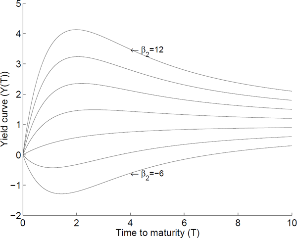
For τ = 1, β0 = 0 and β1 = −1, we get

$Y(T)=1-(1-{\beta }_2)(1-exp(-T))/T-{\beta }_{2}exp(-T).(11.159)$

For β2 ∈ [−6,12] and T up to 10 years, the yield curves in Figure 11.4 are obtained. It is seen that the Nelson-Siegel model is able to fit a large variety of yield curves, increasing, decreasing and humped yield curves.

Another way to see the shape of the attainable yield curves is to interpret the terms in (11.159) as measuring the strength of the short, medium and long-term components (or segments) of the yield curve. The contribution of the long term component is β0, that of the short term components is β1 and β2 indicates the contribution of the medium term component. This is depicted in Figure 11.5. Thus estimation of the yield curve is merely a question of obtaining parameter estimates that weigh these three contributions simultaneously.

It can be shown that the Nelson–Siegel model does not give rise to arbitrage-free prices, but there are arbitrage free extensions (Christensen et al. [2011]). Nevertheless the Nelson–Siegel method is used today in a number of financial institutions.

11.7 Notes

For an introduction to the large variety of bonds on the Danish market (Jensen et al. [1994] and Christensen [1995]). In these notes, we have only considered univariate models for the short rate of interest and the forward rates. Extensions to multivariate SDEs may be found in Strickland [1996], Jørgensen [1994], Duffie [1996], Brennan and Schwartz [1979], Longstaff and Schartz [1992], Chen [1996] or the original paper by Heath et al. [1992] with respect to forward rates.

Multivariate affine models are considered in an excellent article by Duffie and Kan [1996]. See Björk [2009] for the derivation of the term structure equation using the modern approach. A more thorough analysis of the CIR model from a PDE point of view is given by Feller [1951].

Whether one chooses to build the bond pricing framework on the short rate of interest or the forward rate, the pricing equations turn out to be parametrized in (t, T) with T being the fundamental parameter in spite of the fact that the initial discussion showed that a more natural choice would be the time-to-maturity T − t. The latter approach is taken in the socalled Musiela parametrization (Björk [1996] for further details and references). See Wilmott et al. [1995] and Brigo and Mercurio [2006] for two different but excellent overviews of interest rate and credit derivative products.

11.8 Problems

Problem 11.1

Consider a coupon bond with N payments c = (c1,...,cN)′ at discrete time instants T = (T1,..., TN)′ and maturity date T = TN.

1. Show that the price of a coupon bond is given by

   $P(t,c,T)={\displaystyle \sum _{i=1}^n}{c}_{i}P(t,T_i)(11.160)$

   by direct application of (11.2).

Problem 11.2

1. Show that the following applies for t ≤ s ≤ T

   $P(t,T)=P(t,s)exp\left(-{\displaystyle \underset{s}{\overset{T}{\int }}}f(t,u)\text{d}u\right)(11.161)$

   and in particular

   $P(t,T)=exp\left(-{\displaystyle \underset{s}{\overset{T}{\int }}}f(t,u)\text{d}u\right).(11.162)$

Problem 11.3

Show that the zero-coupon bond and forward rate term structures are equal for the time-to-maturity τ*, where the zero-coupon term structure reaches its highest value in the following special cases:

1. The Merton model.
2. The Vasicek model.
3. The Cox–Ingersoll–Ross model.

Can you give an intuitive or financial explanation of this property?

Problem 11.4

Consider an affine term structure.

1. Show that the duration D(t, T) is −B(t, T).
2. Show that the convexity C(t, T) is B2(t, T).

Problem 11.5

Consider the CIR model

$\text{d}r(t)=\kappa (\theta -r((t))\text{d}t+\sigma \sqrt{r(t)}\text{d}W(t).(11.163)$

Assume that the term structure is affine, i.e.,

$P(t,T)=e^{A(\tau )+B(\tau )r(t)}.(11.164)$

1. Determine A(τ) and B(τ).

Problem 11.6

Consider the Ho–Lee model

$\text{d}r(t)=\theta (t)\text{d}t+\sigma \text{d}W(t),(11.165)$

which gives rise to an affine term structure

$P(t,T)=e^{A(t,T)-B(t,T)r(t)}.(11.166)$

1. Determine A(t,T) and B(t,T).
2. Determine the forward rates f(0, T).
3. Determine the forward rates f(t, T).

4. Use the relation

   $P(t,T)=exp\left\{-{\displaystyle \underset{t}{\overset{T}{\int }}}f(t,u)\text{d}u\right\}(11.167)$

   to show that

   $P(t,T)=\frac{P(0,T)}{P(0,t)}exp\left\{-\frac{{\sigma }^{2}Tt}{2}(T-t)-\sigma (T-t)W(t)\right\}.(11.168)$

5. Determine the spot interest rate r(t) from f(t, ·).
6. Use this result to eliminate the Wiener process in (11.168).

Problem 11.7

Consider the Nelson—Siegel model described in Section 11.6.3.

1. Show (11.158).
2. Determine ${\displaystyle \underset{T\to \infty }{lim}}Y(T)$ and ${\displaystyle \underset{T\to 0}{lim}}Y(T)$. Use these limits to explain why it is reasonable to impose the constraints β0 > 0 and β0 + β1 > 0.
3. Plot (11.156) and (11.157) as a function of T.

4. Show that the curvature component of (11.158) reaches its maximum for T = τ.

   In Svensson [1994], an additional term, β3(T/τ2)exp(−T/τ2), τ2 > 0, is added to (11.157) to add flexibility to the model and to allow for better fits to real data. The resulting model is called the Nelson-Siegel-Svensson model.

5. Compute (Y(T), defined by (11.156), for the Nelson-Siegel-Svensson model.

6. Determine ${\displaystyle \underset{T\to \infty }{lim}}Y(T)$ and ${\displaystyle \underset{T\to 0}{lim}}Y(T)$ for the Nelson-Siegel-Svensson model.

   In Gilli et al. [2010] and Annaert et al. [2013] some of the problems related to estimating the parameters in the Nelson–Siegel and Nelson—Siegel-Svensson models are discussed.

1In order to remember this we have chosen to use the notation r(t) as opposed to rt in Chapter 10.

2The precise behavior at the barrier depends on the relation between the drift and diffusion parameters (Feller [1951]).

3http://www.bis.org.