
Chapter 14
Inference in partially observed processes
14.1 Introduction
This section concentrates on filtering (state estimation) and prediction theory related to state space models. There are several reasons for considering state space models. The primary reason is probably that the process described by the system equation of the state space model is a (first-order) Markov process (assuming that the Itō interpretation is used). Furthermore, the state space formulation contains a measurement equation which allows for a rather flexible structure of the observations (aggregation of the state variables, missing measurements, etc.).
More specifically we shall assume that the system is described by the continuous-discrete state space model, which will be introduced in the next section. The evolution of the state vector of the model will be described by a vector Itō stochastic differential equation, which is the system equation of the state space model. The observations are taken at discrete time instants, and the measurement equation of the state space model describes how the observations are obtained as a function of the states plus some measurement noise.
In many references on filtering for SDE (as for instance Øksendal [2010]) a continuous-continuous time setup is used. The continuous-discrete-time setup is, however, the most relevant setup in practice, since the changes of the system most often take place in continuous time, whereas the observations are obtained at discrete time instants.
Assume that we want to estimate the state of the system at time t based on measurements until time tk. Then this chapter describes some estimation methods which might be useful:
- State interpolation (t < tk)
- State filtering (estimation) (t = tk)
- State prediction (t > tk)
In particular the methods are needed for estimating parameters in the stochastic differential equations.
14.2 Model
In the most general case we shall assume that the system equation is the vector Itō stochastic differential equation
dX(t)=μ(X(t),U(t),t)dt+σ(X(t),t)dW(t)(14.1)
with {W(t)} being a vector Wiener process with incremental covariance Q(t), and U(t) some input vector valued function. The observations yk are taken at discrete time instants, tk, as described by the measurement equation:
yk=h(xk,uk,θ,tk)+ek(14.2)
where {ek} is a vector Gaussian white noise process independent of W(t), for all t, k, and ek ~ N(0, Sk). (The super- or subscript k is a shorthand notation for tk.)
However, occasionally a scalar version of the above model will be considered. From the deterministic settings it is well known that a solution to a differential equation ∂X(t)/∂t = μ(t,X(t)) with initial condition X(0) exists and μ(t, X(t)) is unique if μ(X(t), t) satisfies theLipschitz conditions in X(t), and is bounded with respect to t for every X(t). Similar conditions are relevant for the SDE in Equation (14.1).
Condition 14.1 (Lipschitz and growth conditions).
Suppose the real functions μ and σ, and initial condition X(0), satisfy the following conditions. The functions J and a satisfy the uniform Lipschitz conditions in x:
||μ(x2,t)−μ(x1,t)||≤K||x2−x1||,||σ(x2,t)−σ(x1,t)||≤K||x2−x1||.
The functions μ and σ satisfy Lipschitz conditions in t on [t0, T]:
||μ(x,t2)−μ(x,t1)||≤K|t2−t1|,||σ(x,t2)−σ(x,t1)||≤K|t2−t1|.
Furthermore, assume that the drift and diffusion term satisfies
||μ(x,t)||2+||σ(x,t)||2≤K(1+||x||2).(14.3)
The initial condition X(0) is a random variable with E[||X(0)||2] < ∞, independent of {W(t), t ∈ [t0, T]}.
If condition 14.1 is satisfied then {X(t)} is a Markov process, and, in the mean square sense, is uniquely determined by the initial condition X(0) (Jazwinski [1970], Øksendal [2010]).
The Lipschitz condition in x guarantees that the equation has a unique solution, while the Lipschitz condition in t guarantees that the solution does not explode, i.e., it is a restriction on the growth of the functions. The latter is illustrated in the following example.
Example 14.1 (Growth restriction on μ).
Consider the deterministic differential equation
dx(t)dt=x(t)2.(14.4)
The general solution is
x(t)1C−t,(14.5)
where C is an arbitrary constant. For the initial condition x0 = 1 the solution is
x(t)11−t(14.6)
which is defined only for 0 ≤ t < 1.
Given this initial condition no solutions exists for t ≥ 1, and we see that the solution explodes for t ↑ 1.
14.3 Exact filtering
In the general case exact filtering requires that the whole distribution is used.
14.3.1 Prediction
We start by analysing the Scalar case to build some intuition, before proceeding to the multivariate case.
14.3.1.1 Scalar case
Let us first consider the scalar SDE
dX(t)=μ(X(t),t)dt+σ(X(t),t)dW(t).(14.7)
From a previous chapter it is well known that (given the Itō interpretation, which will be adapted in the following) X(t) is a Markov process. Being Markov, the process is then characterized by the density p(x, t) and the transition probability p(x(t)|x(s)) (s < t), and the key issue is to find out how this transition probability propagates in time. Note that we use the shorthand notation p(x(t)|x(s)) instead of the more correct notation p(x(t), t|x(s), s).
Let us consider the process at times s < t < t + δt. For a Markov process we have the Chapman—Kolmogorov equation
p(x(t+δt)|x(s))=∫∞−∞p(x(t+δt)|x(t))p(x(t)|x(s))dx(t)(14.8)
where it is used that p(x(t + δt)|x(t), x(s)) = p (x(t + δt)|x(t)) because of the Markov property.
Using the Chapman—Kolmogorov in a Taylor expansion of p(x(t)|x(τ) (see Maybeck [1982a] p. 192—196) we get the Fokker—Planck equation (F-P) (or the forward Kolmogorov equation)
∂p(x(t)|x(τ))∂t=−∂p(x(t)|x(τ))μ(x,t)∂x+12∂2p(x(t)|x(τ))σ2(x,t)∂x2(14.9)
for the Scalar case (14.7).
Example 14.2 (Einstein's 1905 paper on Brownian motion).
As an example of the F-P equation and its solution we might consider the 1905 paper of Einstein where he treated the Brownian motion. Take μ = 0 and σ = 2D in Equation 14.7. Then Einstein proved that the density p conditioned on a known initial state x0 satisfies
∂p(x(t)|x(τ))∂t=D∂2p(x(t)|x(τ))∂x2.(14.10)
This is the heat diffusion equation with diffusion coefficient D. Notice that this equation is a special case of the F-P Equation 14.9.
It is well known and easy to check that the solution is
p(x(t)|x(0)=0)=1√2π2Dtexp(−x2(t)2(2Dt))(14.11)
which is the Gaussian density with mean zero and variance 2Dt.
14.3.1.2 General case
For the general state space model (14.1)—(14.2) the evolution of the probability density p(X(t)|ℱk), t ∈ [tk, tk+1 [is described by Kolmogorov's forward equation or the Fokker—Planck (F-P) equation:
dp(x(t)|ℱ(0)=L(p)dt(14.12)
where
L(⋅)=−n∑i=1∂(⋅μi)∂xi+12n∑i,j=1∂2(⋅(σQσT)ij)∂xixi(14.13)
is the forward diffusion operator (Jazwinski [1970], Maybeck [1982b]). This is the evolution between observations. The initial condition, at tk, is p(xk|ℱ(0)). We assume this density exists and is once continuously differentiable with respect to t and twice with respect to x.
Example 14.3 (The F-P equation used on a linear system).
Consider the linear system
dX=A(t)X(t)dt+σtdW(t)(14.14)
where W(t) is a Wiener process with incremental covariance Q(t).
If we assume that the initial density is Gaussian, then the density for X(t) will be Gaussian. Hence also the conditional densities will be Gaussian. The Fokker—Planck equation gives the following equation for the conditional density
∂p∂t=−ptr(A(t))-∂pT∂xA(t)x+12tr(σQσT∂2p∂x2).(14.15)
Since it is known that the solution is the Gaussian density, the (conditional) characteristic function for the solution can be written as
ϕ(u,t)=∫∞−∞exp(iuTx)p(x)dx(14.16)=exp(iuTmt−12uTPtu)(14.17)
where mt and Pt are the conditional mean and covariance, respectively.
Using a similar Fourier transformation of the Fokker-Planck equations and comparing the terms with the terms in (14.16) we get (after some calculations — see McGarty [1974]):
dm(t)dt=A(t)m(t),(14.18)dP(t)dt=A(t)P(t)+P(t)A(t)T+σ(t)Q(t)σ(t)T.(14.19)
This gives the exact solution for linear systems driven by a Wiener process, but for non-linear systems it is not sufficient to consider only the conditional mean and covariance. However, some approximative solutions involving only the first and second moment will be considered in some subsequent sections.
14.3.2 Updating
Now, we also assume that the observation mapping h, given in (14.2), is continuous in x and in t, and bounded for each tk with probability 1.
An integrating of the Kolmogorov's equation yields p(xk+1|ℱ(tk)). When a new measurement is available at tk+1, the distribution can be updated through Bayes' rule yielding p(xk+1|ℱ(tk+1)). This is used in turn as the new initial condition for Kolmogorov's equation.
The updating equation is therefore
p(xk|ℱ(tk))=p(yk|xk)p(xk|ℱ(tk−1))∫[xk]p(yk|ξ)p(ξ|ℱ(tk−1))dξ.(14.20)
Note that the denominator is simply p(yk|ℱ(tk−1)). Conceptually, we now have the analytical tool to solve the state filtering problem, but in practice the tool is in general not feasible. Therefore some approximations or truncated expansions are often used. One possibility is to concentrate on only the first moments of the entire distribution. This will be considered in the next section.
14.4 Conditional moment estimators
What we have achieved so far is that by defining a suitable integral (Itō integral), we presented a solution to the transition (prediction) distribution of the state (Kolmogorov's equation). Then we used the observation equation and the Bayes' rule to update the distribution after each measurement. Thus, we have the whole posterior probability distribution of the state. We often like to reduce the distribution to some numbers that are much easier to work with.
A very common approach is to look only upon the first and second moments of the posterior distribution. In fact, it can be shown that choosing the posterior mean of the state as an estimate for the value of the state, we have minimized a Bayesian risk. More precisely, we have the following theorem:
Theorem 14.1 (Optimal state estimation).
The estimate that minimizes E[(X(t)−ˆxt)TW(X(t)−ˆxt)], is the conditional mean. Here W is some positive definite weight matrix and ˆxt afunctional on ℱ(tk) for t ≥ tk.
Proof. See Jazwinski [1970].
14.4.1 Prediction and updating
Let Ek[·] denote the conditional mean of [·] given ℱ(tk). Also, let ˆxt|k and Pt|k denote the conditional first and second (central) moments given ℱ(tk), respectively.
The time propagation (prediction) and the update of the conditional mean and covariance are described by the following theorem:
Theorem 14.2 (Conditional moment estimators).
Assume the conditions required for the derivation of the conditional density in (14.12) and (14.20).
Prediction: Between observations, the conditional mean and covariance satisfy
dˆxt|kdt=ˆμ(X(t),t)(14.21)dPt|kdt=^xtμT−ˆxt|kˆμT+^μxTt−ˆμˆxTt|k+^σQσT(14.22)
for t ∈ [tk, tk+1[, where ^[⋅]=E[⋅|ℱ(tk)], i.e., the conditional mean with respect to ℱ(tk).
Updating: When a new observation arrives at tk we have
ˆxk|k=E[xkp(yk|xk)|ℱ(tk)]E[p(yk|xk))|ℱ(tk)](14.23)Pk|k=E[xkxTkp(yk|xk)|ℱ(tk)]E[p(yk|xk))|ℱ(tk)]−ˆxk|kˆxTk|k.(14.24)
Predictions ˆxt|k and Pt|k, with t > tk, based on ℱk, also satisfy (14.21) and (14.22).
Proof. Is found, e.g., in Maybeck [1982b].
The theorem provides the complete solution to the state filtering problem, but an evaluation of the conditional expectations requires knowledge of the entire conditional density. In order to obtain a computationally realizable filter, some approximations must be made. First, we restrict our attention to a special, though at the same time, very important class of models, namely, linear models.
14.5 Kalman filter
The exact solution of the state filtering problem for linear dynamic models, i.e., models described by stochastic differential equations of the form
dX(t)=A(U(t),t)X(t)dt+B(U(t),t)dt+σ(t)dW(t)yk=C(uk,tk)xk+D(uk,tk)uk+ek
where W(t) is a Wiener process with incremental covariance Q(t), and ek is the Gaussian white noise, given by the Kalman Filter.
Theorem 14.3 (Continuous-discrete Kalman filter).
The Kalman filter (KF) consists of recursive equations for updating and prediction. In the following the dependencies of time and external input of the matrices in the Kalman filter equations have been suppressed for convenience.
The formulas for predicting the mean and covariance of the state-vector and observations are given by,
dˆxt|kdt=Aˆxt|k+But,(14.25)dPt|kdt=APt|k+Pt|kAT+σQσT,t∊[tk,tk+1[.(14.26)
The initial conditions are ˆx1|0=μ0 and P1|0 = V0.
Having the moments for predicting the state vector, the mean and covariance of the next observation are readily found:
ˆyk+1|k=Cˆxk+1|k+Duk+1,(14.27)Rk+1|k=CPk+1|kCT+S.(14.28)
The formulas for updating the mean and the covariance are given by the following equations:
ˆxk|k=ˆxk|k−1+Kk(yk−ˆyk|k−1),(14.29)Pk|k=Pk|k−1−KkRk|k−1KTk,(14.30)Kk=Pk|k−1CTR−1k|k−1.(14.31)
Proof. See e.g., Maybeck [1982b].
14.6 Approximate filters
The derivation of the standard Kalman filter is done under the assumption of linearity and Gaussian distributions. However, it can be shown using Hilbert space formalism, (Appendix A) that these predictions and updates are the optimal linear updates, even when the distributions are non-Gaussian.
14.6.1 Truncated second order filter
Let us for simplicity first consider the scalar SDE
dX(t)=μ(X(t),t)dt+σ(X(t),t)dW(t).(14.32)
Furthermore, let ϕ(·) be some function of x(t). It is well known that E[ϕ(X)]=∫∞−∞ϕ(x)p(x,t)dx. Hence
ddtE[ϕ(X)]=∫∞−∞ϕ(x)∂p∂tdx=∫∞−∞ϕ(x)∂∂x(pμ)dx+12∫∞−∞ϕ(x)∂2∂x2(pσ2)dx=E[dϕ(x)dxμ(X(t),t)]+12E[∂2ϕ(x)∂xσ2(X(t),t)] (14.33)
where the first equality follows from the F-P equations for (14.32), whereas the second one follows by using partial integration.
Equation (14.33) is fundamental for finding the truncated second order filter. Choosing ϕ(x) = x, then (14.33) implies that m(t) = E[X(t)] and
dm(t)dt=E[μ(X(t),t)]≈μ(m(t),t)(14.34)
which describes the time propagation of the conditional mean, or the conditional first moment when the process X(t) and the conditional mean m(t) are similar. Note that the time propagation depends on the entire distribution for x. Now, by taking ϕ(x) = x2 and again using (14.33) we get
ddt=E[x2](t)=E[2X(t)μ(X(t),t)]+E[σ2(X(t),t)].(14.35)
A first-order approximation of this expression is given by
ddt=E[x2](t)≈2m(t)μ(m(t),t)]+2Pt∂μ(mt,t)∂x.(14.36)
Since d(m2t)=2mtdm(t)dtdt≈2m(t)μ(m(t),t)dt we finally get the prediction equation for the conditional variance
ddtPt=2(E[X(t)μ(X(t),t)]−mtμ(m(t),t)+E[σ2(X(t),t)](14.37)≈2Pt∂μ(mt,t)∂x+σ2(mt,t)(14.38)
where the second line is the first-order linearized dynamics.
These equations for the conditional (on ℱ(tk)) mean and variance are valid for times t > tk. These prediction equations are generalized to the vector case in (14.21)—(14.22).
The prediction equations of the truncated second order filter are now obtained by approximating the various expectations above by using a Taylor series representation, truncating to second order and taking conditional expectations for the resulting terms:
dmtdt=μ(mtt)+12Pt∂2μ(mt,t)∂x2(14.39)dPtdt=2Pt∂μ(mt,t)∂x(14.40)+(σ2(mt,t)+Pt(∂∂xσ(mt,t))2+Ptσ(mt,t)∂2∂x2σ(mt,t))
which clearly is a system of non-linear differential equations.
14.6.2 Linearized Kalman filter
In the general non-linear case, a very common approach is based on linearization of the functions around a nominal trajectory. Thus, we can use the Kalman filter derived for the linear model. The matrices are calculated by A(W(t), θ, t) = ∂μ/∂x|x=x*, B(W(t), θ, t) = ∂μ/∂u|x=x*, etc., where x* is some reference signal.
There are different ways to calculate the reference trajectory. One way is integrating the state equation after setting the noise equal to zero. This method, called the linearized Kalman filter, will only converge if the noise levels are sufficiently small.
14.6.3 Extended Kalman filter
Consider now the slightly simplified, vector-valued, non-linear state space model
dX(t)=μ(X(t),t)dt+σ(t)dW(t)(14.41)
with {W(t)} being a Wiener process with incremental covariance Q(t). The observations yk are taken at discrete time instants, tk,
yk=h(xk,tk)+ek(14.42)
where {ek} is a Gaussian white noise process independent of W(t), for all t, k and ek ~ N(0, Sk).
Compared to the state space model (14.1)—(14.2) the simplification is mainly obtained by assuming that the diffusion term is independent of the state vector.
The extended Kalman filter (EKF) is a better choice for the linearization trajectory. The EKF uses the current estimate of the state in the linearization and applies then a Kalman filter to the resulting linearized model.
Theorem 14.4 (Continuous-discrete extended Kalman filter).
For the continuous-discrete state space model (14.41)—(14.41) the (linearized) prediction equations are
dmtdt=μ(mt,t),(14.43)dPt|kdt=F(mt,t)Pt|k+Pt|kFT(mt,t)+σQσT,(14.44)F(mt,t)=∂μ∂x|x=mt,(14.45)
for t > tk. Remember that denotes the conditional mean. The update at time tk is given by
The conditional expectations are calculated as if xk were Gaussian with mean and covariance .
Proof. See Jazwinski [1970]. It is seen that, e.g., the prediction equations are obtained as a simplification of the truncated second order filter.
Performance improvement for the extended Kalman filter may be obtained by local iterations (over a single sample period) on nominal trajectory redefinition and subsequent re-linearization.
The algorithm called the iterated extended Kalman filter (IEKF) is obtained by iterating the equations for the measurement update, where we replace Equation (14.29) with the following iterator
with , and Kk = Kk(ηi−1), iterated for i = 1, ..., l, starting with , and terminating with the result . The algorithm is illustrated on Figure 14.1. Linearizing often leads to significant improvements when the observations are informative; cf. Lindström et al. [2008].
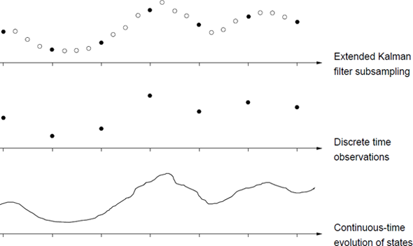
The continuous-time and discrete time scales considered for the iterated extended Kalman filter.
14.6.4 Statistically linearized filter
In this approach, we approximate μ(X(t), t) by a linear approximation of the form
which has the minimum mean square error
for all t ∈ [tk−1, tk[, where W is a positive definite weight matrix. Calculating the partial derivatives of (14.52), with respect to μ0(t) and F(t) and setting them to zero, we get by using the notation of Theorem 14.2
where notation indicated that the quantity is an approximation of E[μ(X(t), t)X(t)T], with Pt|t being the conditional covariance of X(t).
Similarly for the measurement equation:
with the coefficients statistically optimized to get
The issue now is the computation of and H(tk). They all depend upon the conditional probability density function of x, which in general is not available. We therefore assume that the density is Gaussian.
We obtain the statistically linearized filter, with the following equations for the time propagation
with F(t) given by (14.54), and the conditional expectations involved calculated under the assumption that xt is Gaussian with mean and covariance Pt|k. The measurement update at time tk is given by
The conditional expectations are calculated as if xk were Gaussian with mean and covariance Pk|k−1. The equations for the gain and covariance are the same as those for the EKF, with the changes F(t) replacing and H(tk) replacing .
14.6.5 Non-linear models
Let us first introduce the most general class of models which will be considered, namely the non-linear models where the system equation is the Itō equation
where the state vector x is d-dimensional. The r-dimensional input u is assumed to be known. The functions μ and G are continuous and given up to the unknown parameter θ ∈ Θ ⊆ ℝp, and Wt is a standard Wiener process. The solution X(t) of the Itō equation is a Markov process. The initial state X(0) is assumed to be Gaussian with mean m0 and covariance P0.
The observations are taken at discrete time instants, tk, as described by the measurement equation
where y is m-dimensional and e is a Gaussian white noise process independent of w, and ek ~ Nm(0, Sk(θ)). (The super- or subscript k is a shorthand notation for tk.)
Note that the state dependence of the σ matrix is discarded, which makes the state filtering much simpler than described in Section 14.3. Furthermore, it will be shown that if the actual system contains a state dependent diffusion term, then a transformation approach might be used to transform the equations into an equivalent state space model where the diffusion term is independent of the state. It is equivalent in the sense that it contains the same parameters and relates the same input and output.
14.6.6 Linear time-varying models
If the model is linear in the state variable, then a considerable simplification is obtained in the estimation procedure. Hence, consider the linear time-varying stochastic differential equation
The measurement equation is
The specifications of the noise terms are the same as for the non-linear models in the previous section.
There are different approaches leading to the model (14.65)—(14.66). The model may be formulated directly in this form. Alternatively the model may typically be formulated as a linear model, only with coefficients varying according to some known external signal. Yet another approach leading to this class of models is a linearization of the general Itō differential equation around some reference signal x*. In this case the matrices are calculated by A(W(t), θ, t) = ∂μ/∂x|x=x*, B(W(t), θ, t) = ∂μ/∂u|x=x*, etc.
14.6.7 Linear time-invariant models
A further simplification is obtained if the model is linear and time-invariant. Hence, the system equation is
and the measurement equation is
Note that the matrices in (14.67)—(14.68) are now constant, and thus independent of t and W(t).
14.6.8 Case: Affine term structure models
The price of a zero-coupon bond valued in the affine term structure framework, (Section 10.4.2), is given by an exponentially affine function of latent variables such as the infinitesimal interest rate r(t), stochastic volatility v(t), etc.
This form makes it easy to estimate the latent factors within the Kalman filter framework by defining the measurement equation using log prices
while the latent processes are given by diffusion models for the short term interest rate and stochastic volatilty.
14.7 State filtering and prediction
In order to estimate the embedded parameters of the various continuous-discrete time state space models introduced in the previous section, we need the one-step prediction errors of the measurements and the associated covariance.
The one-step prediction error or innovation is
where the predictor, g(tk, θ, yk−1, uN) is a function of old outputs, the parameters and the inputs. In the following the input sequence uN is skipped for convenience, but since we are considering off-line methods the inputs are assumed to be known.
The issue now is to formulate the predictor corresponding to the various models. For the Gaussian maximum likelihood method, which will be considered in subsequent sections, we also need the covariance of the predictions, for evaluation of the likelihood function. For non-Gaussian maximum likelihood methods higher order moments or even the whole distribution p(yk|ℱk−1, θ) is needed.
To solve these problems, we must establish the conditional density for xk conditioned on the measurements p(xk|ℱk) up to and including time tk. If this objective can be accomplished, then various estimators can be defined, optimal with respect to some specified criterion, such as the conditional mean or the conditional mode.
Gaussian maximum likelihood methods will be used for parameter estimation. For linear models the Gaussianity follows directly from the Wiener and Gaussian noise assumption, whereas for non-linear models the Gaussian method is an approximation.
As indicated in Eq. (14.72) a prediction of the state vector is needed in order to predict the output. For the different state space models this prediction is provided by either an ordinary or an extended Kalman filter. Let us first consider the ordinary Kalman filter, which can be used for linear models.
14.7.1 Linear models
14.7.1.1 Linear time-varying models
It is known from Section 14.5 that for linear models the ordinary Kalman filter provides an exact solution of the filtering problem. Hence, for the linear models (14.65)—(14.66) and (14.67)—(14.68), the updating formulas are
and the prediction formulas for the conditional mean and covariance of the state vector are
Then the one-step prediction of y and the associated covariance are finally obtained
The dependencies of time and external input of the matrices in the Kalman filter equations have been suppressed for convenience. This implementation of the Kalman filter thus involves the solution of a set of ordinary differential equations between each sampling instant.
14.7.1.2 Linear time-invariant models
If the matrices in the system equation, i.e., A, B and σ, are time invariant, then it is possible to find an explicit solution for (14.25) and (14.26), by integrating the equations over the time interval [tk, tk+1 [and assuming that ut = uk in this interval, thus obtaining
where the matrices Φ, Γ and Λ are calculated as
and τ = tk+1 − tk is the sampling time. This implementation of the Kalman filter thus involves the calculation of the exponential of a matrix. In the time invariant case this is done only once for each set of parameters.
14.7.2 The system equation in discrete time
Let us first consider the linear and time invariant case.
Assuming that the sample interval is [tk, tk + τ[= [tk, tk+1[the discrete time model corresponding to the continuous-time model (14.67) is in the same way given as
Under the assumption that W(t) is constant in the sample interval the sampled version can be written as the following discrete time model in state space form
where
On the assumption that W is a Wiener process, vk(τ) becomes Gaussian distributed white noise with zero mean and covariance
where is the incremental covariance of the Brownian motion; cf. the Itō isometry. If the sampling time is constant (equally spaced observations), the stochastic difference equation can be written
where the time scale now is transformed such that the sampling time becomes equal to one time unit.
If the time dependence is slow compared to the dominating eigenvalues of the system, this implementation of the Kalman filter may also be used for time varying systems, by evaluating (14.88) for each sampling instant, assuming that A, B and σ are constant within a sampling time. This solution requires less computations and is more robust than integrating (14.25) and (14.26) (Moler and van Loan [1978], van Loan [1978]).
14.7.3 Non-linear models
Let us now consider the non-linear model defined by (14.63)—(14.64). In this case the extended Kalman filter is used as a first-order approximative filter. Being linearized about , the state and covariance propagation equations have structures similar to the Kalman filter propagation equations for linear systems. Hence, we are able to reuse the numerical stable routines implemented for the Kalman filter.
The necessary modifications of the equations in the previous section are the following. The matrix C is the linearization of the measurement equation,
and A is the linearization of the system equation,
and Φ is the discrete system matrix calculated as a transformation of A, (Equation (14.88)). The prediction of the output, Eq. (14.78), is replaced by
The formulas for prediction of mean and covariance of the state-vector are normally given by
where A is given by (14.92) and t ∈ [tk, tk+1[. In order to make the integration of (14.94) and (14.95) computationally feasible and numerically stable for stiff systems, the time interval [tk,tk+1[is subsampled and the equations are linearized about the state estimate at the given subsampling time. For the state propagation the equation becomes
where [tj, tj+1[is one of the subintervals of the sampling interval [tk, tk+1[, and we assume that the sampling interval has been divided in ns subintervals. In these derivations only the state dependency is given for simplicity. Equation (14.96) is a linear ordinary differential equation which has the exact solution
where τs = tj+1 − tj = τ/ns, and τ is the sampling time. Correspondingly the equation for the state covariance becomes
which is similar to (14.81). The algorithm to solve (14.94) and (14.95) uses and as starting values for (14.98) and (14.99) and then performs ns iterations of (14.98) and (14.99) simultaneously. This algorithm has the advantage of being numerically stable for stiff systems and still computationally efficient, since the fast and stable routines of the linear Kalman filter can be used.
14.8 Unscented Kalman Filter
The approximations in Section 14.6 can sometimes be a bit crude, and/or can be complicated to compute in practice. Specifically, the covariances can be poorly approximated, and may even become negative definite under certain circumstances which would lead to a diverging filter.
An alternative is to use the unscented Kalman filter (UKF) which computes second order (third if the density is Gaussian (Julier and Uhlmann [1997], Julier et al. [2000])) accurate approximation of the first and second central moments; see also Nørgaard et al. [2000] for a related idea called central difference Kalman filter.
The idea is to approximate the joint distribution of two random vectors X and Y when
where g : ℝn ↦ ℝm is some non-linear function. This can of course be computed using standard quadrature methods, but the unscented transform is doing it in a computationally convenient way.
The unscented transform approximates the joint density of X and Y according to
This is rather straightforward (perhaps a bit tedious though) to compute. Define the Cholesky factorization of the covariance matrix P as
This will be used to compute the sigma point and associated weights as
and
where λ = α2(n + κ) − n. These parameters can be used to tune the filter (α and κ control the spread of the sigma points while β is related to the distribution of X), but a common choice is α = 10−3, κ = 0 and β = 2.
Each sigma point is propagated through the non-linear function g according to
The parameters in Equation (14.102) are then computed as
The unscented transform, taking a function g, a mean m and covariance P, will be denoted UT (g, m, P) for the remainder of the text.
The resulting filter is then given by iterating the prediction and update steps. Assume that the discrete time model is given by
Starting from a Gaussian density at time k, i.e., xk ∊ N(mk|k,Pk|k), the prediction step is then given by
where the last line is needed to correct for the fact that the function f is ignoring the additive noise.
The update step is similar, computing predictions as
where the variance of the measurement noise S is added to the variance of y in the second line. No noise is added to the covariance, however, as the measurement noise is independent of the latent state xk. Finally, the state is updated using the standard Kalman filter equations
The near optimality (the equations are optimal in the class of linear updates) of these equations is proved using Hilbert space methods in Appendix A.
The unscented Kalman filter is generally seen as more robust than the extended Kalman filter (Van Der Merwe [2004], Lindström and Strålfors [2012], Wiktorsson and Lindström [2014]). The unscented Kalman filter has also been extended further to continuous-discrete models in Sarkka [2007].
14.9 A maximum likelihood method
This section describes how the embedded parameters of the linear and nonlinear continuous-discrete state space models can be estimated using a maximum likelihood method. We stress that much of these results presented in this Section carries over to the unscented Kalman filter, even though the results are presented for a simple class of processes.
First it is assumed that the evolution in time of the states of the system is described by the diffusion process
where X is d dimensional, and the process W(t) is assumed to be a Wiener process with the incremental covariance . Furthermore it is assumed that X(0) is Nd(m0, P0).
As described in Section 14.7.2 the evolution of the states in discrete time is under some conditions exactly described by the following discrete time stochastic process
where are random d × 1 vectors, and are non-random r × 1 input vectors, and x0 is Nd (m0, P0) and . The random vector x0 and the system noise v1,..., vN are all assumed to be stochastic independent. Here, {Φk} and {Γk} are non-random d × d and d × r matrices, respectively.
The relation between the continuous-time matrices and the discrete time matrices are described in Section 14.7.2.
If we assume that the functions A, B and are continuous and given up to the unknown parameter , then we can write down the likelihood function for θ
where is the density for the distribution of x0 and the density for the conditional distribution of xk given xk−1. Hence
However, often we do not observe the state vectors x0, x1,..., xN directly. We assume that the state vector is only partially observed and possibly with measurement errors. We assume that the measured quantities are given by the measurement equation
where {Ck} and {Dk} are non-random matrices of dimensions m × d and m × r (m ≤ d). For the measurement error we assume that ek ~ Nm(0, Sk), k = 0,..., N. Finally, we assume that x0, v1,..., vN, e0, e1,..., eN are stochastically independent.
In the following let all the non-random elements in (14.124) and (14.128) including m0 and the unknown variance parameters be given up to some unknown parameter θ ∊ Θ ⊆ ℝp where Θ is some compact set. Furthermore, recall that
is the information set containing all the observations up to and including time tk.
The likelihood function is
where p0(y0|θ) is the density for the distribution of y0 and pk|k−1(yk|ℱk−1, θ) the density for the conditional distribution of yk given ℱk−1. Hence
Note that due to the incomplete observation of the state variable we now need to condition on all previous observations and not only the previous observation as in (14.127).
Furthermore, note that the unknown vector m0 can be a part of θ. Even the conditional log-likelihood function (conditioned on y0) for θ
depends on m0. This is also clear from the fact that m0 is needed as an initial value for calculating pk|k−1(yk|ℱk−1; θ) (see for instance the filtering approach described in Section 14.7.1). In the literature, however, the initial value is often chosen at random (Pedersen [1993]).
Since vk, ek and x0 are all Gaussian distributed, the conditional density pk|k−1(yk|ℱk−1; θ) is also Gaussian. The Gaussian distribution is completely characterized by the mean and covariance.
Hence, in order to parameterize the conditional distribution, we introduce the conditional mean and covariance as
respectively. It is noticed that (14.133) is the one-step prediction and (14.134) the associated covariance. Furthermore, it is convenient to introduce the one-step prediction error (or innovation)
Using (14.132)—(14.135) the conditional log-likelihood function becomes
where m is the dimension of y.
The conditional mean and covariance are calculated recursively by using the state filtering techniques described previously in Section 14.7.1.
The maximum likelihood estimate (ML estimate) is the set , which maximizes the likelihood function. Since it is not, in general, possible explicitly to optimize the likelihood function, a numerical method has to be used.
An estimate of the uncertainty of the parameters is obtained by the fact that the ML estimator is asymptotically normally distributed with mean θ and covariance
where the matrix H is given by
However, this is not necessarily true if the filter is not exact. Then QuasiMaximum likelihood asymptotics should be used instead of this approximation.
An estimate of D is obtained by equating the observed value with its expectation and applying
The above equation can be used for estimating the variance of the parameter estimates. The variance also serves as a basis for calculating t-test values for test under the hypothesis that the parameter is equal to zero. The correlation between the estimates is readily found based on the covariance matrix.
The maximum likelihood method described in this section is implemented in a software tool called CTSM (Kristensen et al. [2004]).
14.10 Sequential Monte Carlo filters
Recent advances in computational resources have made Monte Carlo methods viable. Sequential Monte Carlo methods (or particle filters) approximate the filter problems by Monte Carlo sampling and resampling; see Lopes and Tsay [2011], Creal [2012], for an overview.
14.10.1 Optimal filtering
The optimal filtering problem for general state space models is non-trivial, as we will see soon. Let us consider a model where the latent system equation is a Markov process, and hence is defined by the transition kernel
We remind the reader that this is not a severe restriction as, for example, an AR(p) model (which is non-Markovian) can be rewritten as an VAR(1) model with dimension p which is a Markovian model. Other models, like fractional AR processes, can also be approximated by Markovian models.
Observations are thought of as noisy and/or incomplete readings of the latent state vector, formally expressed through the measurement kernel
The observations are assumed to be independent, when conditioning on the latent state vector. We are now ready to compute (at least theoretically) the log-likelihood for the observations
where y1:n−1 is used as shorthand notation for y1..., yn−1.
The likelihood for observation yn conditional on the history can be expressed as
where we used the law of total probability and the conditional independence of the observations. The likelihood for observation can be seen as the measurement kernel, weighted by the prediction of the latent state pθ (xn|y1:n−1).
The prediction can in turn be computed using the law of total probability and the Markov property, according to
where we see that the prediction is derived from the transition kernel and the filter density, pθ (xn−1|y1:n−1). What remains is to compute the filter density, which is found by using Bayes' formula, arriving at
This closes the recursion if we also know the initial distribution for the latent Markov process, pθ (x0), as shown in Algorithm 1. The algorithm is similar to the Kalman filter, but this should not to surprise anyone as the Kalman filter is a very well-known special case of the general optimal filtering equations.
Algorithm 1 Optimal filtering recursion
Require: p(X0),p(Xn|Xn−1),p(Yn|Xn)
for n = 1 : N do
Compute prediction using Equation (14.145)
Update using Equation (14.147)
end for
14.10.2 Bootstrap filter
The main problem with Equation (14.145) and (14.147) is the difficulties to solve them in practice. There are two well-known cases where we can solve them: the linear Gaussian case (leading to the Kalman filter) and the Hidden Markov model with a discrete and finite state space (as all integrals will be finite sums).
The main idea behind the bootstrap filter is to approximate the general state space model with a Hidden Markov model. This allows for very general results concerning stability and convergence of the approximate filters (Künsch [2005]).
Replacing a measure p(x) with a Monte Carlo sample from that measure (sometimes referred to as the empirical measure, cf. theoretical statistics) will introduce some unwanted variability, but it will also make computations easier. It is worth noticing that the empirical measure can be written, using the law of total probability as
where p(x|k) = δ(x − x(k)) and p(k) = ωk.
Computing the expectation (assuming that the expectation is finite)
is potentially very difficult whereas the Monte Carlo approximation
is a trivial to computation. The law of large numbers ensures that the approximation converges (a.s.) as K → ∞. The convergence is more complicated when the samples are dependent, but the results still hold under rather general conditions (Douc and Moulines [2008]).
It is possible, given some minor modifications, to solve the optimal filtering problem (cf. Section 14.10.1) for arbitrary distributions when they are replaced with empirical samples. It should not be a problem (direct sampling, accept-reject, etc.) to sample from the initial distribution, generating .
What remains in Algorithm 1 is to alternate between prediction and updating. Predicting is simple as
A common choice is simply to sample from leading to the empirical measure
Updating is less trivial, as the empirical filter measure is given by
It should be clear to the reader that this new empirical measure only takes values where there is a Dirac measure, meaning that the expression can be simplified as follows
where
which ensures that the weights sum to unity.
A practical problem, which can be shown theoretically, but is more easily seen in a “trial and error” Monte Carlo simulation, is that the weights tend to become unevenly distributed after only a few iterations, i.e., the largest weight will be close to one and the rest close to zero. This is called particle degeneracy, as the original K particles act as there is only one particle.
However, this is solved by resampling, thus creating a new empirical measure with equal weights. That prevents serious particle degeneracy as there will be plenty of particles with non-zero weight even if the weights are updated unequally.
The Sequential Importance Sampling with Resampling (SISR) algorithm (also known as the bootstrap filter) is presented in Algorithm 2, where we also consider using an importance sampler in order to improve the performance of the Monte Carlo approximations.
Algorithm 2 Sequential Importance Sample with Resampling
Require: p(xx0),p(xn|xn−1),p(yn|xn)
At time n=0, draw and set
for n = 1 : N do
Draw and compute
Normalize the importance weights to get
Draw (with replacement) K indices to get anew equally weight empirical measure with particle .
end for
14.10.3 Parameter estimation
A major problem with particle filters is that the straightforward approximation of the log-likelihood is only a pointwise approximation. It can also be shown that the approximation is discontinuous in the parameter space, due to the resampling of the particles (Figure 14.2). That graph shows the log-likelihood function for the model
where ek and vk are standard Gaussian random variables, and a = 0.6 in the example. The simulation is based on N = 500 observations and K = 1 000 particles. Still, the Monte Carlo approximation is sharing the same global features of the exact log-likelihood, and the Monte Carlo error can be controlled by using sufficiently many particles.

Log-likelihood function for a partially observed AR(1) model (N = 500 observations) with true parameter a = 0.6. The maximum likelihood estimate is shown with a pentagon, and 95% confidence intervals are shown with the dotted line. The solid line is the log-likelihood function computed using a Kalman filter, and the dots are 3 independent estimates of the log-likelihood function using a particle filter, each using K = 1 000 particles.
It is argued in Spall [2005] that derivative-free optimization methods, such at the Nelder-Mead simplex (e.g., fminsearch in MATLAB®), often are quite capable of optimizing a noisy function, often reaching a point close to the true optima of the function.
Other methods include Expectation-Maximization methods (Cappé et al. [2005] and references therein), but this requires the smoothing distribution (as opposed to the filter distribution). Simple (typically slightly biased) approximations include fix lag smoothers (Olsson et al. [2008]) while Briers et al. [2010], Fearnhead et al. [2010], Douc et al. [2011] present computationally efficient algorithms for asymptotically unbiased approximations of smoothing distribution. The EM algorithm will have to be replaced by either a Monte Carlo EM (MCEM) algorithm (Cappé et al. [2005]) or a Stochastic Approximation EM algorithm (Ditlevsen and Samson [2014] for an example).
An alternative is to augment the state space with the parameters. This is in general not a consistent estimation technique, but Ionides et al. [2006, 2011] derived a version where consistency is proved. Their algorithm was later refined in Lindström et al. [2012] and fine-tuned in Lindström [2013b].
14.11 Application of non-linear filters
14.11.1 Sequential calibration of options
Non-linear Kalman filters have successfully been used to calibrate vanilla S & P 500 index options in Lindström et al. [2008]. The most common method for calibrating options to market data today is some non-linear weighted least squares estimator
where cMarket (Si,Ki, ri, τi) are the market price that depends on the underlying asset Si, strike level Ki, interest rate ri, and time to maturity τi and λi, are weights (it is statistically optimal to relate the weight of an observation to the inverse of the variance of the measurement error for that observation — i.e., observations that we trust are given more weight than the others).
There are two main (implicitly related) problems with this approach:
- The parameter estimates are noisy,
- Old data are typically discarded, as only the most recent data are used.
Old data are discarded as adaptivity is sought, but this comes at a price. If yesterday's data are of little use today, then today's data will be of little use tomorrow! Lindström et al. [2008] rewrites the calibration problems as a filtering problem, augmenting the latent states with the parameter vector
This decomposes the change of the option prices into changes in the underlying state variables (i.e., the index level), changes in the parameters (which is captured by the random walk dynamics) and pure noise due to the ask-bid spread.
It is sometimes worthwhile to include the underlying asset in the calibration as well. The algorithm was extended further in Lindström and Guo [2013] where it was shown that quadratic calibration strategies are found for free when using this algorithm. A computational refinement of the simultaneous calibration and hedging algorithm was presented in Wiktorsson and Lindström [2014]. The extended calibration mode is given by the measurement equations
and the latent states
The performance of the non-linear filter, when changing some parameters, is evaluated in Figure 14.3 for the Heston model.

Adaptive calibration of the Heston model to simulated data, when parameters are changing. The true parameter value is the solid line, non-linear filter estimate is the dotted line and the triangles are daily non-linear least squares estimates.
The non-linear filter is able to track the changing parameters (smooth variations are tracked well, jumps in the parameters are assimilated after a few consecutive observations), while the non-linear least squares using only the current observations are quite noisy but generally adapt somewhat quicker.
The performance of the sequential calibration algorithm, when calibrating a Heston model to S & P 500 data between late 2001 and 2003, is presented in Figure 14.4. The cloud of non-linear least squares estimates is again scattered around the filter estimates.
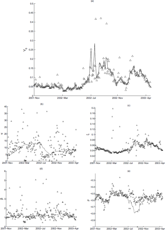
Calibration of the Heston stochastic volatility option valuation model to S & P 500 index options.
14.11.2 Computing Value at Risk in a stochastic volatility model
Value at risk is a popular measure of risk; cf. Embrechts et al. [2005], Hult et al. [2012]. It is well known that volatility varies over time (cf. Chapter 1), so some sort of stochastic volatility model is needed. The standard GARCH family of model (Section 5.5.2), is very popular, but is unable to cope with unexpected events as the volatility (according to the model) at time n + 1 is perfectly known at time n. An alternative is the stochastic volatility model (Section 5.5.3),
where zn and en are independent standard Gaussian random variables.
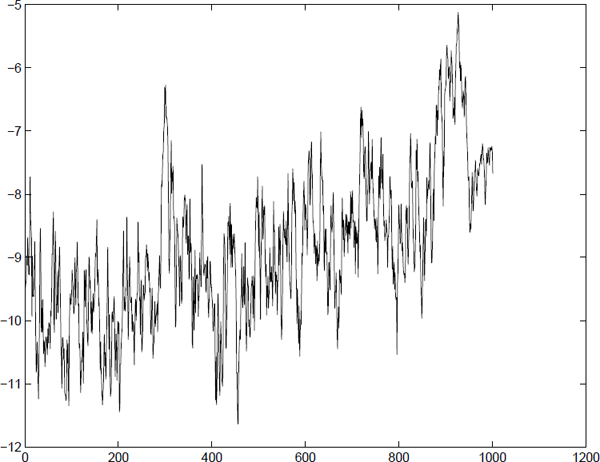
A stochastic volatility model was fitted to OMXS30 (a Swedish stock index consisting of the 30 largest companies listed) with data from March 30th, 2005 to March 6th, 2009. The parameters were found by optimizing the likelihood using MATLAB'S fminsearch routine, which is a (derivative free) Nelder-Mead simplex method. The returns and estimated log-variance are presented in Figure 14.5 and 14.6.

More interesting is the computation of the Value at Risk (VaR) statistic. It is defined as the quantile
This is rather easy to compute as we know that the measurement kernel is Gaussian and we have a particle representation for p(xny1:n−1). It follows that
We know from the model specification that the measurement kernel is Gaussian with zero mean and variance . Computing the VaR simply comes down to numerically solving Equation (14.165) with the measurement kernel plugged into Equation (14.168). The result in shown in Figure 14.7 where 61 returns were below the VaR level when computing VaR at the 5% level.

Value at Risk computed for the 0MXS30 between March 30th, 2005 and March 6th, 2009. Approximately 5% of the returns are lower than the computed VaR at the 5% level.
This deviation is not statistically significant as an approximate interval of the number of observations that is expected to end up below the VaR level is (36,64) observations.
14.11.3 Extended Kalman filtering applied to bonds
In this section, we utilize the modelling framework from Chapter 14 consisting of the state space model (14.1) and the measurement equation (14.2). In this particular case, the state space model will describe the spot interest rates and the measurement equation will be the solution of the bond pricing equation (11.66) (plus some additive white noise). This framework allows us to estimate both the parameters in the state space model and the implied interest rates. The term implied is used, because the estimated interest rates (obtained by utilizing the extended Kalman filter) are the interest rates implied by the bond prices and not the interest rates that are quoted in the financial markets.
It should be noted that this framework is only applicable for Gaussian interest rate models, although they may be multivariate. Thus it is not possible without some modification to use this method for, e.g., the Cox–Ingersoll–Ross model. This restriction may be overcome by introducing the transformation of the diffusion term with that was discussed in Section 13.4. In addition, it is a necessary requirement that an explicit solution to the bond pricing equation (11.66) is available.
For the large class of models, where this solution is not available, one has to resort to, e.g., Monte Carlo simulation. In this case, the measurement equation is estimated on the basis of a bond price which is obtained by a Monte Carlo simulation of the expectation in (11.66). Due to the Feynman–Kac representation theorem, the bond price may also be obtained by solving the PDE associated with (11.66) numerically. Although both methods are conceptually simple, they are extremely demanding from a computational point of view. We will not go into more details here, but a number of references are listed in the Notes.
Let us sketch the procedure that we wish to use:
- Given an interest rate model (or state space model),
- the bond pricing formula (11.66) is solved analytically. The solution constitutes a measurement equation.
- Input series are designed to model the payout of coupons and the time to maturity
- This is implemented in a program, and
- the model parameters are implemented using the conditional maximum likelihood method discussed in Chapter 14.9.
Data description
The method is applied to time series of daily observed prices for Danish Government Bonds1 listed in Table 14.1 for the period 2/8-94 to 8/9-95. Each time series consists of 282 observations. These bonds pay out a coupon once a year and the size of the coupon c is constant throughout the lifetime of the bond. At maturity the bond pays out a coupon c and the amount C, where C = DKK 100 for Danish Government Bonds.
The considered Danish Government Bonds
ISIN |
Bond |
Maturity |
|---|---|---|
DK0009915035 |
9% Danske Stat St. Laan |
15/11 1996 |
DK0009915548 |
9% Danske Stat St. Laan |
11/11 1998 |
DK0009916439 |
9% Danske Stat St. Laan |
15/11 1995 |
DK0009917916 |
6% Danske Stat St. Laan |
10/2 1996 |
DK0009918054 |
5.25% Danske Stat St. Laan |
10/8 1996 |
DK0009918567 |
6.25% Danske Stat St. Laan |
10/2 1997 |
Certain conventions are associated with trading of Danish Government Bonds: A “bond year” consists of 12 months each containing 30 days. Therefore months with 31 days are cut one day short and February is extended by 2 days (or 1 day in leap years). This is not taken into account in this thesis. Furthermore the day of settlement is 3 days later than the day of agreement, but this is not deemed to be relevant as we are modelling the actual bond prices.
Bonds are not traded during weekends, so bond prices for weekend days are not available, but the model should take these “missing” prices into account as the underlying stochastic process that generates the spot interest rate evolves in continuous time. The extended Kalman filter is used to predict the missing prices using the dynamics of the interest rate model (rather than replacing bond prices for the weekends by some interpolation scheme). Hence each time series is expanded to cover a period of 402 days.
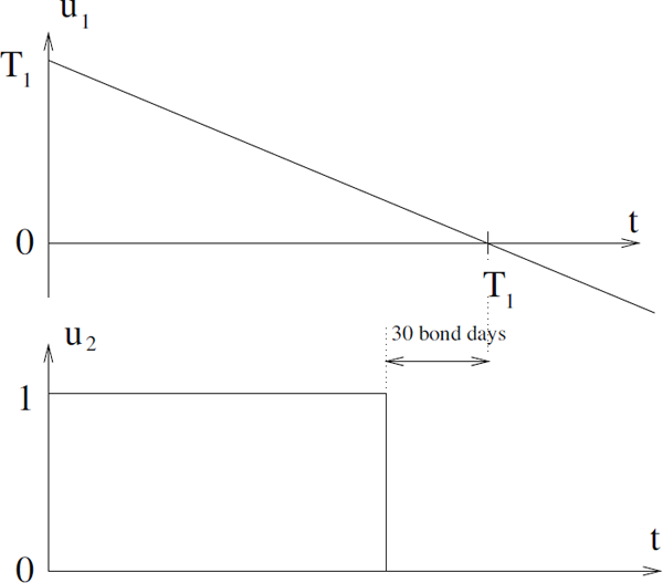
Should a bond be traded less than 30 “bond days” prior to the coupon being payed to the holder of the bond. Hence the bond price is reduced by the coupon value c 30 prior to the maturity date. Furthermore the time-to-maturity T − t in the measurement equation has to be incorporated into the estimation procedure. These conventions have been implemented by incorporating two designed input variables U = [u1 u2] in the measurement equation as illustrated in Figure 14.8, where u1 models the time to the first coming payout T1 − t and u2 models the payout of a coupon. If bond prices were available for a longer period of time spanning n coupon payouts, n similar input variables should be incorporated.
14.11.4 Case 1: A Wiener process
A simple Wiener process is considered initially
where σ(r, t) = σ implies constant volatility. The solution to (14.169) is given by
where r(t0) is the implied interest rate at time t0.
Using this model, it may be shown that the price of a coupon bond should satisfy the equation
or, by adding a noise term to account for measurements errors,
where {ek} is a white noise with zero mean and variance .
Estimation results for the Wiener process. The values given in parentheses are asymptotic t-test values for the hypothesis that the parameter is equal to zero. It is seen that does not differ significantly from zero, i.e., there are no measurement errors. Similar results are obtained by reestimation without the variance parameter .
ISIN |
||||
|---|---|---|---|---|
DK0009916439 |
0.06562 (39.9924) |
1.1941e-4 (12.3497) |
0.1311e-8 (0.2282) |
16.7% |
DK0009917916 |
0.06649 (46.1670) |
0.9004e-4 (14.8825) |
0.1223e-8 (0.7197) |
14.3% |
DK0009918054 |
0.06748 (47.4841) |
0.7502e-4 (13.5571) |
0.1686e-8 (1.0042) |
12.8% |
DK0009918567 |
0.06927 (32.0052) |
0.7801e-4 (12.4275) |
0.4450e-8 (1.4287) |
12.8% |
14.11.5 Case 2: The Vasicek model
Again, we consider the Vasicek model
where α, γ and σ are constants, and W(t) is a standard Wiener process.
In the literature, it is reported that it is very difficult to estimate the adjustment parameter α, unless a long time series is available (i.e., at least several times longer than the half life of the process implied by α parameter). A long time series might give rise to other problems on its own, namely that the time series structural breaks, regime shifts or other nonlinear phenomena render the model 14.173 unappropriate. We had serious difficulties in obtaining reasonable and consistent estimates of the model parameters with the parameterisation of the original model suggested by Vasicek [1977].
In Jørgensen [1994], an alternative parameterisation of the model is suggested, but the bond pricing framework is not worked through with this new parameterisation:
The complete framework will be reported in this section. The bond pricing framework for this spot interest rate model is established by making the transformations
in the framework introduced in Vasicek [1977].
This yields the bond pricing formula
The conditional mean and variance of the interest rate is
Especially, in the limits, we get
It is seen from (14.181) that the variance is zero at maturity t = T, i.e., the instantaneous rate of return is exactly the spot interest rate r. This is in compliance with the deterministic nature of the partial differential equation that the individual bond prices must satisfy and the adjacent boundary condition P(T, T, r) = 1.
The results in Table 14.3 are obtained.2 The estimates of θ are not shown as the obtained estimates did not differ significantly from zero. Therefore the estimation procedure was repeated for each time series with η fixed at zero. This also applies for the variance of the measurement noise.
Results for the Vasicek model
5548 |
8054 |
8567 |
|
|---|---|---|---|
4.44167E-04 (13.7703) |
5.70140E-04 (94.5229) |
5.11133E-04 (1.5214) |
|
0.0728404 (49.1246) |
0.0675208 (43.9797) |
0.0693201 (44.9230) |
|
2.27742E-07 (12.8445) |
2.06625E-07 (12.7473) |
2.15661E-07 (13.1400) |
|
12.4308% |
12.7734% |
12.7109% |
|
χ2 (α) |
47.77 (44.1%) |
59.06 (11.2%) |
49.17 (38.6%) |
ρ |
A first examination of the listed correlation matrices shows that the parameter estimates are uncorrelated, and, hence, each parameter may be interpreted independent of the others.
The estimates of η are very small, and similar across time series, but it should be kept in mind that η is a continuous-time parameter. The estimates of r(t0) seem reasonable and are well determined. Based on these estimates, the annual relative volatility σr is determined for each time series. As discussed previously, the σr should be within the range 10–20%, and this is indeed the case.
14.12 Problems
Problem 14.1
Let
be a vector of jointly multivariate Gaussian random variables.
- 1. Derive the distribution for p(X|Y).
2. Show that
Problem 14.2
1. Derive the conditional distribution for using a Kalman filter, assuming some Gaussian density for m0, e.g., p(m0) = N(μ0,Σ0).
Hint: Design a latent process such that the distribution of mt can be found.
- 2. Relate the result to prior knowledge in statistics.
1The ISIN number is an international coding used for bonds. Only the last four digits will be used in the following.
2Unless stated otherwise, the values in parentheses are asymptotic t-test values for insignificant parameters.