Chapter 10

Stochastic interest rate models

In this chapter, we shall provide a catalogue of a number of well-known models of interest rates as it is important to be familiar with these often referenced models and, in particular, their properties. The main focus is on univariate stochastic differential equations or one-factor models as they are called in the financial literature because only one state variable (or factor), r(t), is used to describe variations in the interest rate.

Conceptually r(t) is the continuously compounded interest rate of risk-free financial securities, which was introduced in Section 2.3. Thus r(t) denotes the instantaneous interest rate or the spot rate obtained by investing in a riskless security in the time interval [t, t + dt].

Application of univariate SDEs is based on the assumption that the spot rate contains all relevant information about the financial market, the expectations of the market participants (agents), etc. For some time interest rates were assumed to follow a random walk, which implies that the mean and variance structures are independent of time and the current level of interest rate, i.e., there are no level effects. The analysis of interest rates in the problems and exercises has shown that this is clearly not the case.

Empirical studies have shown that at least 3—4 state variables are required to explain the variations in observed interest rates (e.g. Braes and Larsen [1989], Nielsen [1995], Piazzesi [2010]). The former reference uses multivariate statistics (principal component analysis, etc.) and the latter uses the concept of the fractal dimension of an attractor in state space and other methods from deterministic chaos theory. The first component will typically capture parallel shifts in the interest rate, the second difference between short and long term interest rates, while the third will capture how intermediate rates will move contrary to the movements of the short and long term rates.

In Section 2.3, we assumed that the interest rates were deterministic, but our discussion of e.g., the CIBOR time series in Section 2.4 showed that interest rates are indeed stochastic.

As we shall see interest rates models are inherently important for pricing and hedging financial derivatives which should be clear from the definition of a money market account (Definition 2.2). Recall that this is used to discount future payments of some contingent claim to determine its present value. In particular for fixed income securities, i.e., securities whose future payoffs are contingent on future interest rates, it is important to model interest rates. As we have argued previously, interest rates are obtained from bond prices, and we will briefly discuss this relation in order to view interest rate models in their context. The bond pricing framework and a detailed study of the so-called term structure of interest rates shall be postponed to later.

This chapter is organized as follows: Section 10.1 describes models that give rise to normally distributed interest rates. Section 10.2 extends these models to non-Gaussian interest rates. Section 10.3 extends the last section by allowing the drift and diffusion parameters to be time-dependent functions. Section 10.4 provides a brief introduction to a very broad class of multivariate SDEs or multifactor models, where additional variables are used to model the interest rate. It also considers stochastic volatility models, where one aims at modelling the volatility by considering a function of the volatility as a state variable.

10.1 Gaussian one-factor models

We fix a standard Wiener process W(t) restricted to some finite time interval [0, T] on a given probability space $(\Omega ,ℱ,\mathbb{P})$ augmented by the natural filtration ${\{ℱ(t)\}}_{t\ge 0}$. This establishes the structure of information in the considered models. We assume that r(t) is $ℱ(t)$-adapted and that it does not explode.

10.1.1 Merton model

The simplest, non-trivial model for spot interest rates was suggested by one of the pioneers in continuous-time finance, Robert Merton (Merton [1993]) for an overview of his work. The Merton model is a Wiener process with a constant drift, i.e.,

$\text{d}r(t)=\theta \text{d}t+\sigma \text{d}W(t)(10.1)$

where θ and σ are some constants and r(0) is a deterministic initial value. The model is sometimes called the arithmetic Brownian motion.

This model was considered in Example 8.2, where we found that

$\begin{array}{cccc}\hfill E[r(t)]& =& r(0)+\theta t\hfill & \hfill (10.2)\\ \mathrm{Var}[r(t)]& =& {\sigma }^{2}t.\hfill & (10.3)\end{array}$

We see that there is a drift in the mean and that the variance grows with time. The solution to (10.1) is given by

$r_r=r(0)+\theta t+\sigma W(t).(10.4)$

As the Wiener process generates normally distributed stochastic variables, it is clear that rt is also normally distributed with the parameters given in (10.2). Thus the Merton model (10.1) does not exclude negative interest rates, which renders the model unapplicable for empirical work. It is also unclear why the interest rate should have a constant drift at all times.

10.1.2 Vasicek model

The constant drift and unlimited variance of the Merton model (10.1) is not found in the classical model attributable to Vasicek1 (Vasicek [1977]).

The Vasicek model is given by

$d{r}_t=(\theta +\eta r(t))\text{d}t+\sigma \text{d}W(t)(10.5)$

where η < 0, θ and σ are some constants, r0 is a deterministic initial value and Wt is a standard Wiener process.

The Vasicek model belongs to the class of linear SDEs in the narrow sense considered in Section 8.2.1. Thus the solution is readily found from Theorem (8.6), i.e.,

$r(t)=\left(r(0)+\frac{\theta }{\eta }\right)e^{\eta t}-\frac{\theta }{\eta }+\sigma e^{\eta t}{\int }_0^t{e}^{-\eta s}\text{d}W(s).(10.6)$

This stochastic process is also called the Ornstein-Uhlenbeckprocess. The mean and variance are

$\begin{array}{ccc}\hfill E[r_t]& =\left(r(0)+\frac{\theta }{\eta }\right)e^{\eta t}-\frac{\theta }{\eta },\hfill & \hfill (10.7)\\ \hfill \mathrm{Var}[r_t]& =\frac{{\sigma }^2}{2\eta }(e^{2\eta t}-1).\hfill & (10.8)\end{array}$

It is seen that the process tends to the long term mean value −θ/η, and that the variance is finite for η < 0.

Remark 10.1.

A reparametrization of the Vasicek model, which is often seen in the literature, makes the interpretation of the parameters more clear,

$\text{d}r(t)=\alpha (\beta -r(t))\text{d}t+\sigma \text{d}W(t).(10.9)$

With this parametrization the long term mean is β and the process is said to mean-revert around this mean with the speed of adjustment α.

The Vasicek model is sometimes called an elastic Brownian motion, because the diffusion term is a Brownian motion, but the mean reverting drift term pulls the process towards a long term mean if the short term rate is either above or below the long term mean.

The mean-revertion property of the Vasicek model (10.5) is a very important property of interest rate models, although it may be difficult to estimate the two parameters in the drift term from financial time series.

Clearly the solution to (10.5) is also normally distributed and hence negative interest rates cannot be excluded. The probability of negative interest rates depends on the actual parameter values. This means that if there is a fast speed of adjustment to a relatively high long term mean and a low level of volatility in the market then negative interest rates are clearly highly unlikely, but still negative interest rates can not be excluded.2 Thus the model is not considered as a reasonable model for observed interest rates, but it is nonetheless often used for theoretical work.

Thus we turn our attention to non-Gaussian models in the hope that negative interest rates may be excluded in some of these models. A more important objective is to be able to model the state dependent diffusion, which is, perhaps, the most important property of any interest rate model.

10.2 A general class of one-factor models

In this section, we consider a fairly general one-factor model class, which is attributable to Chan et al. [1992]. With reference to the authors of this article this model is typically called the CKLS model or the generalized Cox-Ingersoll-Ross (CIR) model.3 The CKLS models has also been used to model mean reverting commodities such as electricity (Regland and Lindström [2012]).

The CKLS model class is as follows

$\text{d}r(t)=(\theta +\eta r(t))\text{d}t+\sigma r{(t)}^{\gamma }\text{d}W(t)(10.10)$

where σ denotes a proportional rate of volatility and γ denotes the elasticity of the volatility with respect to spot interest rate changes, and the specification of the drift term is as in the Vasicek model (10.5).

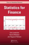
Although this general model specification pertains to the important properties of a mean-reverting drift and a state dependent diffusion term, it is not possible to solve it unless some parameter restrictions are imposed in (10.10). An overview of the important models that belong to this model class is depicted in Figure 10.1. The hierachical structure is well suited for statistical inference. The models obtained by these parameter restrictions are listed in Table 10.1.

Theorem 10.1 (Existence and uniqueness for the CKLS model).

A sufficient condition for the existence and uniqueness of the solution to (10.10) is that the parameters θ = (θ, η, γ) fulfil one of the conditions

1. $\gamma =\frac{1}{2},\theta >\frac{1}{2}{\sigma }^2,\eta <0,$
2. $\gamma \in \left(\frac{1}{2},1\right),\theta >0,\eta \le 0,$
3. $\gamma =1,\theta =0,\eta =\frac{1}{2}{\sigma }^2$, or
4. γ = 1, (θ, η, σ) ∈ ℝ+ × ℝ × ℝ+.

Proof. The conditions are obtained using the scale function (8.8) and Theorem 8.3. See Honoré [1996] for further details.

Remark 10.2.

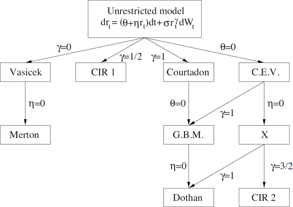
It is duly noted that the case γ > 1 is not covered by the theorem. This will have some implications when estimating parameters in the model. Figure 10.2 presents the US 3 month T-bill between 1983–1995. It can be seen that the variance increases with increasing interest rates.

This empirical property will have some consequences ... The γ parameter will typically be less than one if the interest rate is less than one and greater than one when the interest rate is greater than one. A linear scaling (i.e., using r = 0.05 or r = 5) will often change the estimates!

In the following some comments will be made to each of these models. The Merton and Vasicek models have already been discussed, and they are also members of the CKLS model class.

The Cox-Ingersoll-Ross model (Cox et al. [1985]), is possibly the most popular one-factor model:

$\text{d}r(t)=(\theta +\eta r(t))\text{d}t+\sigma \sqrt{r(t)}\text{d}W(t).(10.11)$

It also has the mean-revertion property and it allows the interest rate level to proportionally influence the variance of the process. Depending on the parameters the process will have a reflecting or an absorbing barrier at zero with the appealing and obvious implication that interest rates will never become negative. The model is for obvious reasons also called the square root process. The CIR model does not belong to the class of linear SDEs in the strong sense considered in Section 8.2, but it may nevertheless be solved in the sense that the marginal distribution of the solution rt is known to be a gamma-distribution (the conditional density is a non-central χ2-distribution).

The Marsh & Rosenfeld model is the well-known geometric Brownian motion (GBM) that has been applied as a model of stock prices in the Black & Scholes model. However, it is highly questionable whether this model conforms to the characteristics that economic intuition would normally lead one to expect from an interest rate model, as the interest would either grow towards infinity or converge towards zero (at least under the ℙ measure).

The Courtadon model is a combination of the Vasicek and Dothan model, and it belongs to the class of linear SDEs in the strong sense considered in Section 8.2.

The Cox (& Ross) model is also called the constant elasticity of variance (CEV) model, and it allows for a very general modelling of the volatility. However, the drift term does not seem reasonable.

An empirical comparison of these models shall be made in the following chapters on parameter estimation in stochastic differential equations.

10.3 Time-dependent models

In this section, we introduce time-dependent counterparts to some of the models from the last section. The financial reasons for allowing the parameters in, e.g., (10.10) to be time-dependent will be discussed later. It is, however, rather obvious that a better fit to observed time series may be obtained by allowing the parameters to be time-dependent.

10.3.1 Ho–Lee

The Ho-Lee model is simply obtained by allowing the drift term in the Merton model (10.1) to be time-dependent, i.e.,

$\text{d}r(t)=\theta (t)\text{d}t+\sigma \text{d}W(t).(10.12)$

It can be shown that θ(t) can be chosen such that a perfect fit to all zero-coupon prices can be obtained (Section 11.3.2).

10.3.2 Black–Derman–Toy

The Black-Derman-Toy model is obtained by allowing the parameters in the Marsh & Rosenfeld model to be time-dependent, i.e.,

$\text{d}r(t)=\eta (t)r(t)\text{d}t+\sigma (t)r(t)\text{d}W(t)(10.13)$

where both the drift θ(t) and the diffusion σ(t) are allowed to be time-dependent. This will make the model more flexible, but also more prone to overfitting. The BDT model is often implemented in a trinomial tree.

10.3.3 Hull–White

The Hull-White model exists in two versions, namely as extensions of either the Vasicek model (10.5) or the Cox-Ingersoll-Ross model. For brevity, we will only list the latter, i.e.,

$\text{d}r(t)=(\theta (t)+\eta (t)r(t))\text{d}t+\sigma (t)\sqrt{r(t)}\text{d}W(t).(10.14)$

This makes the model prone to overfitting as three functions are used to fit a finite number of observations, but the model is still not able to account for the dynamics of the term structure; cf. HJM models (Section 11.4).

10.3.3.1 CIR++ model

A rather clever special case of the Hull-White model is the so-called CIR++ model (Brigo and Mercurio [2001, 2006] for a detailed analysis). The idea is to introduce a time varying function such that a simple model (here a CIR process) plus that time varying function provides perfect fit to the term structure.

Consider the model where the interest rate is a combination of a diffusion process x(t) and a deterministic function of time ɸ(t)

$r(t)=x(t)+\varphi (t).(10.15)$

We focus on the case when x(t) satisfies a CIR process. It is then clear that all we need to know in order to obtain a perfect fit to the current term structure is knowledge about the model implied term structure of x(t). The time varying function ϕ(t) can then be chosen such that perfect fit to the term structure is obtained (Brigo and Mercurio [2006] for details on theory and implementation).

10.4 Multifactor and stochastic volatility models

An alternative approach to obtain more flexibility than in the constant parameter univariate case is to introduce additional state variables, such as the price level, the inflation level, the money supply, etc.

One way to introduce the so-called multifactor models is to assume that the spot interest rate is given by a function r(t) = R(t,X(t)), where the n-dimensional state variable X(t) is described by the multivariate Itō stochastic differential equation

$dX(t)=\mu (t,X(t))\text{d}t+\sigma (t,X(t))\text{d}W(t)(10.16)$

where R: [0, ∞) × ℝn → ℝ, μ: [0, ∞) × ℝn → ℝ, σ: [0, ∞) × ℝn → ℝn×n are sufficiently well-behaved functions such that existence and uniqueness of the solutions are guaranteed, and W(t) is a n-dimensional Wiener process.

We shall provide a few examples of multifactor models as the theoretical analysis of such models is outside the scope of this book.

First, we extend the CIR model (10.11), which we choose to parametrize slightly different in this case

$\text{d}r(t)=\alpha (\mu -r(t))\text{d}t+\sigma \sqrt{r(t)}\text{d}W(t)(10.17)$

where α is the speed of adjustment and μ is the long term. Although this model contains the level effects discussed previously, it is unreasonable to assume that the long term mean μ should be a constant. Thus we may model the long term mean μ as another CIR model, i.e.,

$\begin{array}{cccc}\hfill \text{d}r(t)& =& \alpha (\mu (t)-r(t))\text{d}t+\sigma \sqrt{r(t)}\text{d}{W}^{(1)}(t)\hfill & (10.18)\\ \hfill \text{d}\mu (t)& =& \beta (\theta -\mu (t))\text{d}t+\delta \sqrt{\mu (t)}\text{d}{W}^{(2)}(t)\hfill & (10.19)\end{array}$

where β, θ and δ are constants, and W(1)(t) and W(2)(t) are two mutually independent standard Wiener processes. A problem with this model specification is that the long term mean process μ(t) is unobservable. Conversely, that also means that bond prices no longer will be perfectly correlated, an empirical fact that is often observed.

Alternatively, we may choose to introduce additional explanatory variables. As an example we consider the model proposed by Pearson and Tong-Schen [1994], i.e.,

$\begin{array}{cc}\text{d}r(t)={\kappa }_1({\theta }_1-r(t))\text{d}t+{\sigma }_1\sqrt{r(t)}\text{d}{W}^{(1)}(t)\hfill & (10.20)\hfill \\ \text{d}p(t)=y(t)p(t)\text{d}t+{\sigma }_{p}p(t)\sqrt{y(t)}\text{d}{W}^{(2)}(t)\hfill & (10.21)\hfill \\ \text{d}y(t)={\kappa }_2({\theta }_2-y(t))\text{d}t+{\sigma }_2\sqrt{y(t)}\text{d}{W}^{(3)}(t)& (10.22)\end{array}$

where κ1, κ2, θ1, θ2, σ1, σ2 and σp (< 1) are positive constants; W(2)(t) and W(3)(t) are correlated Wiener processes but both are independent of W(1)(t). We see that the model is essentially two CIR models supplemented by a process that couples y(t) and p(t). The interesting part is that the state variables have an economical interpretation and may be observed on the market. The state variable r(t) denotes the real interest rate, p(t) denotes the price level and y(t) the inflation rate. This particular model specification has the advantage that it is possible to solve the bond pricing equation as we shall see later.

Empirical studies have shown the interest rate and the volatility of the former are two of the most important factors in the financial markets. If we denote the volatility by V(t), we may, e.g., consider the model proposed by Longstaff and Schartz [1992], i.e.,

$\begin{array}{ccc}\text{d}r(t)& =& \left(\alpha \gamma +\beta \eta -\frac{\beta \delta -\gamma \zeta }{\beta -\alpha }r(t)-\frac{\zeta -\delta }{\beta -\alpha }V(t)\right)\text{d}t\hfill \\ & +& \alpha \sqrt{\frac{\beta r(t)-V(t)}{\alpha (\beta -\alpha )}}\text{d}{W}^{(1)}(t)+\beta \sqrt{\frac{V(t)-\alpha r(t)}{\beta (\beta -\alpha )}}\text{d}{W}^{(2)}(t)(10.23)\hfill \end{array}$

$\begin{array}{ccc}\text{d}V(t)& =& \left({\alpha }^2\gamma +{\beta }^2\eta -\frac{\alpha \beta (\delta -\zeta )}{\beta -\alpha }r(t)-\frac{\beta \zeta -\alpha \delta }{\beta -\alpha }V(t)\right)\text{d}t\hfill \\ & +& {\alpha }^2\sqrt{\frac{\beta r(t)-V(t)}{\alpha (\beta -\alpha )}}\text{d}{W}^{(1)}(t)+{\beta }^2\sqrt{\frac{V(t)-\alpha r(t)}{\beta (\beta -\alpha )}}\text{d}{W}^{(2)}(t)(10.24)\hfill \end{array}$

where the parameters α, β, γ, δ, η and ζ are assumed to be constant.4 Again this particular model parametrization has been chosen because it is possible to solve the bond pricing equation. Furthermore, it may be shown that

$\begin{array}{cc}\text{E}[r(t)]=\frac{\alpha \gamma }{\delta }+\frac{\beta \eta }{\zeta }& (10.25)\\ \text{Var}[r(t)]=\frac{{\alpha }^2\gamma }{2{\delta }^2}+\frac{{\beta }^2\eta }{2{\zeta }^2}& (10.26)\\ \text{E}[V(t)]=\frac{{\alpha }^2\gamma }{\delta }+\frac{{\beta }^2\eta }{2{\zeta }^2}& (10.27)\\ \text{Var}[V(t)]=\frac{{\alpha }^4\gamma }{2{\delta }^2}+\frac{{\beta }^4\eta }{2{\zeta }^2}.& (10.28)\end{array}$

It should be evident that an infinite number of multifactor models may be proposed. So far the criterion in the financial literature has been that it should be possible to determine closed form solutions to the bond pricing equation. However, this may also be done by Monte Carlo simulation or another numerical method such that this criterion is no longer valid. Instead the model that provides the best fit (in some sense) to observed time series should be chosen, but this is clearly a very difficult problem.

10.4.1 Stochastic volatility models

A stochastic volatility model is obtained by using a function of the time-dependent volatility σt as a state variable. These models may be considered as a continuous-time extension of the ARCH models considered in Section 5.5.2, but we shall not go into the mathematical details here.

Empirical studies have shown that $log{\sigma }_t^2$ is an important state variable. As a very general example consider the model

$\begin{array}{cccc}\hfill \text{d}r(t)& =& {\alpha }_1(\mu (t)-r(t))\text{d}t+\sigma (t)r(t{)}^{\gamma }\text{d}{W}^{(1)}(t)\hfill & (10.29)\\ \hfill \text{d}(log{\sigma }^2(t))& =& {\alpha }_2(\beta -log{\sigma }^2(t)\text{d}t+{\xi }_1\sqrt{r(t)}\text{d}{W}^{(2)}(t)\hfill & (10.30)\\ \hfill \text{d}\mu (t)& =& {\alpha }_3(\theta -\mu (t))\text{d}t+{\xi }_2\sqrt{\mu (t)}\text{d}{W}^{(3)}(t).\hfill & (10.31)\end{array}$

We recognize (10.29) as the CKLS model (10.10), where the long term mean μt and the volatility σt are now assumed to be time-dependent. The time dependency of μt is simply modelled by (10.31), namely a Cox-Ingersoll-Ross model (10.11). The interesting part compared to multifactor models is (10.30), where the log volatility $log{\sigma }_t^2$ is modelled with the mean-reversion and state dependent diffusion term that we have come to expect. In particular note that the short term interest rate rt enters the diffusion term in (10.30). Although a clear-cut definition of stochastic volatility models is hard to find, it is (at least) required that (a function of) the volatility is modelled and that the short term interest rate enters this model as in (10.30). Clearly, it is very difficult to determine the parameter restrictions that must be imposed on (10.29)—(10.31) to ensure existence and uniqueness of solutions.

It is an unresolved question whether stochastic volatility models are superior to general multifactor models. The latter aims at modelling the drift by including additional (un)observable variables, whereas the former tends to disregard the drift (except mean-reversion) and focuses on the diffusion. As stochastic differential equations consist of both a drift term and a diffusion term, it is hardly surprising that (at least two) different schools have emerged in the financial community. The reader is encouraged to consider the fundamental difference between these two schools.

10.4.2 Affine Term Structure models

Computational considerations has caused much focus on models that are simple enough to admit a (semi-)closed form expression, and still be flexible enough to capture stylized facts. Here we consider models given by a multivariate jump diffusion

$\text{d}\text{X}(t)=\mu (t,\text{X}(t-))\text{d}t+\sigma (t,\text{X}(t-))\text{d}W(t)+\text{d}J(t)(10.32)$

where J(t) is a compound Poisson process with jump distribution independent of X(t−) having intensity λ(X(t)); cf Section 7.5.

The class of Affine Term Structure models (Piazzesi [2010] for an extensive overview) requires the drift, squared diffusion and jump intensity to satisfy certain conditions under the risk-neutral measure ℚ:

1. The drift μ(t, X(t)) is affine in X(t).
2. The squared diffusion σ(t, X(t))σT(t, X(t)) is affine in X(t).
3. The jump intensity λ (X(t)) is affine in X(t).

It is then possible to show that the price of a zero-coupon bond, formally computed as

$p(t,T)=E^{\mathbb{Q}}\left[e^{{\int }_t^T-r(s)\text{d}s}|ℱ(t)\right],(10.33)$

can be expressed even when the model includes stochastic volatility and stochastic long term mean, etc., as

$p(t,T)=e^{A(T-t)+B{(T-t)}^{T}X(t)}(10.34)$

where A(·) and B(·) are solutions to some differential equations (Piazzesi [2010] for examples). The solution here resembles the Fourier methods in Section 9.6.1, explaining the computational advantages.

The class of Affine Jump Diffusions is very general, including the Vasicek model and the Cox—Ingersoll—Ross model, as well as certain stochastic long term interest rates and stochastic volatility models.

10.5 Notes

Survey articles on interest rate models appear regularly in the financial literature, but we only list a couple, namely Chan et al. [1992] and Strickland [1996]. The first reference introduces an estimation method and compares univariate SDE models empirically. We shall in later chapters discuss and extend their work. The last reference is highly recommendable reading.

A theoretical analysis of interest models (or SDEs in general) may be found in Karatzas and Shreve [1996], Ikeda and Watanabe [1989], but very few results are available on multifactor models.

An excellent discussion of stochastic volatility (SV) models may be found in Musiela and Rutkowski [1997] and Andersen and Lund [1997]. The first reference gives an overview of continuous time models whereas the latter discusses the relation between (G)ARCH models and SV models in detail, and uses the Efficient Method of Moments for parameter estimation (Gallant and Tauchen [1996]).

10.6 Problems

Problem 10.1

Show (10.4).

Problem 10.2

One-factor stochastic interest rate models are very popular for theoretical analysis and thus a huge range of models have been proposed in the financial literature through the years. We have considered the CKLS model class previously. In this problem, we consider a slightly simpler model class (actually a subclass of the CKLS model class) attributable to Courtadon, which gives rise to linear models in the narrow sense. Thus the model may be solved and the first moments may be computed using the methods of Chapter 8.

Consider the one-factor stochastic interest rate model

$\text{d}r(t)=(\theta +\eta r(t))\text{d}t+\rho r(t)\text{d}W(t)r(0)=r_0(10.35)$

where θ, η and ρ are constants, and W(t) is a standard Wiener process.

1. Solve (10.35).
2. Determine the mean E[r(t)]. In particular determine ${\displaystyle \underset{x\to \infty }{lim}}E[r(t)]$.
3. Determine the variance Var[r(t)]. In particular determine ${\displaystyle \underset{x\to \infty }{lim}}\mathrm{Var}[r(t)]$.

Problem 10.3

For θ = 0 in (10.35), we get the geometric Brownian motion

$\text{d}r(t)=\eta r(t)\text{d}t+\sigma r(t)\text{d}W(t)(10.36)$

which, according to Example 8.10, has the solution

$r(t)=r(0)exp((\eta -{\sigma }^2/2)+\sigma W(t)(10.37)$

It appears that the deterministic growth rate in (10.37) is (η − σ2/2) as opposed to the growth rate η in (10.36).

1. DetermineE[eσW(t)].
2. Use this result to show that there is no discrepancy between the expected growth rates in (10.36) and (10.37).

Problem 10.4

Show (10.25) and (10.27).

Problem 10.5

An even more general model of interest rates than (10.10) is considered in Duffie [2010]. It takes the form

$\text{d}r(t)=({\alpha }_{1t}+{\alpha }_{2t}r(t)+{\alpha }_{3t}r(t)logr(t))\text{d}t+{({\beta }_{1t}+{\beta }_{2t}r(t))}^v\text{d}W(t)(10.38)$

where α1t, α2t, α3t, β1t and β2t are time-dependent functions, ν is a constant and W(t) is a standard Wiener process. The reader is encouraged to make a table of the parameter restrictions that must be imposed on (10.38) in order to obtain the models discussed in this chapter.

Assuming that the functions α1t, α2t, α3t, β1t and β2t are constants, we shall now shed some light on the reasonability of the log r(t) term in (10.38).

It might be useful (e.g., for numerical reasons or in order to obtain some kind of variance homogeneity) to consider the process l(t) = log r(t), where lt is described by a Vasicek model

$\text{d}l(t)=(a+bl(t))\text{d}t+\sigma \text{d}W(t).$

Use the Itō formula (8.10) to determine the SDE for r(t) and compare the result with (10.38).

1The original paper Vasicek [1977] is highly recommended reading.

2Nevertheless the normal distribution is often applied as a reasonable model of the height, weight, etc., of a population even though a negative height or weight is impossible.

3The reason for the latter will be clear later.

4We have chosen to use the parametrization from the original paper.