Chapter 6
Kernel estimators in time series analysis
6.1 Non-parametric estimation
Non-parametric methods are widely used in non-linear model building. Such methods are particularly useful if no prior information about the structure is available, since the estimation procedure is free of parameters and model structure (apart from a smoothing constant).
In this chapter we concentrate on kernel estimation. Some other non-parametric methods are based on splines, k nearest neighbour (k-NN) or orthogonal series smoothing. Each method has a specific weighting sequence {Ws(x); s = 1, ..., N}. These weighting sequences are related to each other and it can be argued (Härdle [1990]) that one of the simplest ways of computing a weighting sequence is kernel smoothing. For more information about non-parametric methods see Robinson [1983], Härdle [1990], Silverman [1986], Ruppert et al. [2003] or Hastie et al. [2011].
6.2 Kernel estimators for time series
6.2.1 Introduction
This chapter considers kernel estimation in general and its use in time series analysis. The non-parametric estimators are of particular relevance for non-Gaussian or non-linear time series. From kernel estimates of probability density functions Gaussianity can be verified or the nature of non-Gaussianity can be discovered. Thus non-parametric methods provide information that complements that given, for instance, by higher-order spectral analysis.
Non-parametric estimates of the conditional expectation can be used to detect non-linear structures and to identify a family of relevant time series models. Consider for instance the time series generated by the non-linear model:
Yt=g(Yt−1,...,Yt−p)+h(Yt−1,...,Yt−p)εt.(6.1)
For this model
E[Yt|Yt−1,...]=g(Yt−1,...,Yt−p)(6.2)Var[Yt|Yt−1,...]=h2(Yt−1,...,Yt−p)(6.3)
where it is implicitly assumed that the variance of the white noise process εt is unity in order to avoid identifiability issues.
Thus the non-parametric methods can be used to estimate, e.g., g(y) = E[Yt + 1 |Yt = y] in the simple case p = 1. Using this non-parametric estimate a relevant parametrization of g(·) can be suggested.
Furthermore non-parametric estimates can be used to provide predictors, i.e., estimators of future values of the time series. Use of non-parametric estimators for getting insight in the time-varying behaviour and a complex dependency on exogenous variables will also be considered.
In this section we first introduce the most frequently considered non-parametric estimators for time series, the kernel estimators. Next the kernel estimators are described in more detail. Finally, some examples are given on how to use kernel estimation in time series analysis.
6.2.2 Kernel estimator
Let {Yt; t = 0, ±1, ...} be a strictly stationary process. A realization is given as a time series {yt; t = 1, ..., N}, and that single realization of the process is the basis for inference about the process.
Introduce Zt = (Yt + j1, ..., Yt + jn) and Y*t=(Yt−h1,...,Yt+hm). . In order to simplify the notation we consider the caseY*t=(Yt) in the rest of this section. It is obvious how to generalize the equations.
The basic estimated quantity is
E[G(Zt)|Yt=y]fY(y)(6.4)
where fY is the probability density function (pdf) of Yt and G is a known function.
The estimator of (6.4) is
[G(Zt);y]=(N′h)−1N′∑t=1G(Zt)k(y−Yth)(6.5)
where k(u) is a real bounded function such that ∫ k(u)du = 1, and h is a real number. Here, N′ is some number which corrects for the fact that not all N observations can be used in the sum, typically N′ = N − jn, and k(u) is the kernel function and h is the bandwidth.
Let us consider two examples of using Equation (6.5). In the first example it is illustrated that Equation (6.5) is a reasonable estimator.
Example 6.1
(Non-parametric estimation of a pdf). The pdf of Yt at y is estimated by
ˆfY(y)=[1;y]=1NhN∑t=1k(y+Yth).(6.6)
Assume that Y has pdf f (y), then
f(y)=lim h→012hℙ(y−h<Y≤y+h)(6.7)
when ℙ is the distribution function at Y. An estimator of f(y) is
ˆf(y)=12hn[Number of observations in(y−h;y+h)].(6.8)
Define the rectangular kernel
w(u)={12if|u|<10otherwise.(6.9)
Then the estimator (6.8) can be written as
ˆf(y)=1NN∑t=11hw(y−Yth).
Now consider the general kernel (∫ k(u)du = 1). Then the estimator is
ˆf(y)=1NhN∑t=1(y−Yth)(6.10)
which clearly is equal to Equation (6.6).
Example 6.2
The estimator of the conditional expectation of G(Zt), given Yt = y, is
ˆE[G(Zt)|Yt=y]=[G(Zt);y]1;y=1N′∑G(Zt)k(y−Yth)1N∑k(y−Yth)(6.11)
where [1; y] was found in the previous example.
Of special interest is the case G(Zt) = Yt + 1, where (6.11) estimates E[Yt + 1|Yt = y].
6.2.3 Central limit theorems
Central limit theorems can be established under various weak dependence conditions on the process {Yt}. Let ℱvu be the σ-field of events generated by Yt; u ≤ t ≤ v. Then introduce the coefficient
Definition 6.1
(Strong mixing condition). The process Xt is said to be strongly mixing if αj, → 0 as j → ∞.
The strong mixing condition has been used frequently in the asymptotic theory of estimators for time series; but the condition is often very difficult to check.
Central limit theorems for non-parametric estimators of pdfs of a process {Yt}, as well as of conditional pdfs and conditional expectations at continuity points, are given by Robinson [1983] under the strong mixing condition.
6.3 Kernel estimation for regression
This section describes in more detail the kernel estimation technique. Since the method is useful for non-parametric regression in general, a notation will be used which is related to non-parametric regression; however, the problem is highly related to the estimator in (6.11), and thus also useful in time series analysis.
6.3.1 Estimator for regression
The kernel based non-parametric regression was first proposed by Nadaraya [1964].
Assume that the theoretical relation is
where ε is a white noise, and g is a continuous function.
Given n observations
the goal is now to estimate the function g.
If q = 1, then the kernel estimator for g, given the observations, is
Note that if we compare with Equation (6.5) then G(Zt) = Zt = Yt and the independent variable is now X.
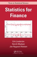
The function k is the kernel, and h is the bandwidth of the kernel, where h → 0 as n → ∞. Various candidate functions for the kernel have been proposed, but it is shown in Härdle [1990] that the parabolic kernel with bounded support, called the Epanechnikov kernel, minimizes the mean square error among all kernels in which the bandwidth is optimally chosen.
The Epanechnikov kernel is given by
Other possibilities are the rectangular, triangular or the Gaussian kernel given by:
These kernels are depicted in Figure 6.1. The Epanechnikov kernel is shown for h = 1, and the Gaussian kernel for h = 0.45.
If we allow q > 1 in (6.14) a kernel of order q has to be used, i.e., a real bounded function kq(x1,..., xq), where ∫ k(u)du = 1.
By a generalization of the bandwidth h to the quadratic matrix h with the dimension q × q the more general kernel estimator for g(X(1),..., X(q)) is
where x = (x1,...,xq) and . This is called the Nadaraya-Watson estimator.
6.3.2 Product kernel
In practice product kernels are used, i.e.,
where k is a kernel of order 1.
Assuming that hi = h, i = 1,..., q the following generalization of the one-dimensional case in (6.14) is obtained
6.3.3 Non-parametric estimation of the pdf
An estimate of the probability density function (pdf) is Robinson [1983]
6.3.4 Non-parametric LS
If we define the weight Ws (x) by
then it is seen that Equation (6.19) corresponds to the local average:
The estimate is actually a non-parametric least squares estimate at the point x. This is recognized from the fact that the solution to the least squares problem
is given by
This shows that at each x, the estimate ĝ is a scaled weighted LS location estimate, i.e.,
6.3.5 Bandwidth
The bandwidth h determines the smoothness of ĝ. In analogy with smoothing in spectrum analysis:
- If h is small the variance is large but the bias is small.
- If h is large the variance is small but the bias is large.
The limits provide some insight:
- As h → ∞ it is seen that as all data are included and given equal weights.
- As h → 0 it is seen that ĝ(x1,...,xq) = Yi for and otherwise undefined (or possibly 0 depending on how ratios of zeros are defined).
6.3.6 Selection of bandwidth — cross validation
The ultimate goal for the selection of h is to minimize the mean square error (MSE)(see Härdle [1990])
where w(...) is a weight function which screens off some of the extreme observations, and g is the unknown function. A solution is the “plug-in” method, where Yi is used as an estimate of in (6.26).
Hence, the criterion is
but it is clear that for h → 0, since when h → 0.
It is clear that a modification is needed! In the “leave one out” estimator the idea is to avoid that () is used in the estimate for Yi. For every data () we define an estimator for Yi based on all data except (). The n estimators (called the “leave one out” estimators) are written
Now the cross-validation criterion using the “leave one out” estimates is
It can be shown that under weak assumptions the estimate of the bandwidth that is obtained by minimizing the cross-validation criterion is asymptotic optimal, i.e., it minimizes (6.26) (Härdle [1990]). An example of using the CV procedure is shown in Figure 6.7.
6.3.7 Variance of the non-parametric estimates
To assess the variance of the curve estimate at point x Härdle [1990] proposes the pointwise estimator given by
where the weights are given as shown previously by
Remembering the WLS interpretation this estimate seems reasonable.
6.4 Applications of kernel estimators
6.4.1 Non-parametric estimation of the conditional mean and variance
Assume a realization of a stochastic process {X1,..., Xn}.
Goal: Use the realization to estimate the functions g(·) and h(·) in the model
For the conditional mean and the conditional variance we shall use the notation
One solution is to use the kernel estimator (other possibilities are splines, nearest neighbour or neural network estimates).
Using a product kernel we obtain
Assuming that E[Xt] = 0 the estimator for V(·) is
If E[Xt] ≠ 0 it is clear that the above estimator is changed to
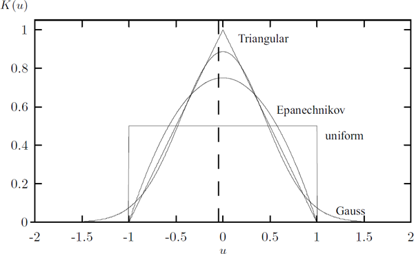
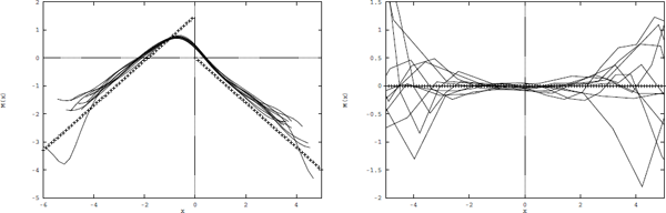
Example 6.3.
Simulations of 10 independent time series have been generated from the following non-linear models:
The first model is a SETAR model with non-linear conditional mean and constant conditional variance whereas the second model is an ARCH model with constant conditional mean and state dependent conditional variance.
A Gaussian kernel with h = 0.6 is used to estimate the conditional mean (Figure 6.2) and variance (Figure 6.3) in order to detect the nonlinearities. The theoretical conditional mean and variance is shown with "+”.
6.4.2 Non-parametric estimation of non-stationarity — an example
Non-parametric methods can be applied to identify the structure of the existing relationships leading to proposals for parametric model classes. An example of identifying the diurnal dependence in a non-stationary time series is given in the following.
Measurements of heat supply from 16 terrace houses in Kulladal, a suburb of Malmö in Sweden, are used to estimate the heat load as a function of the time of the day.
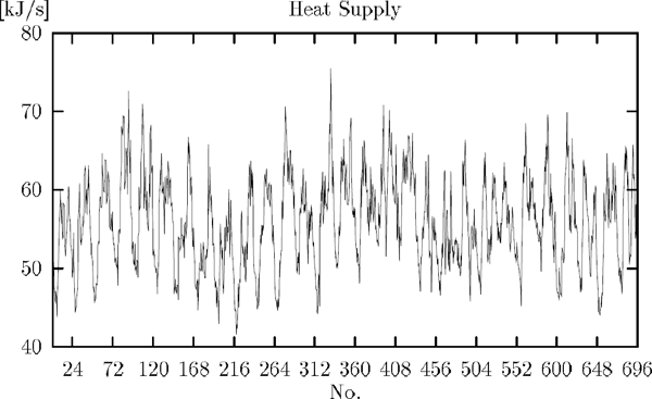
The heat supply was measured every 15 minutes for 27 days. The transport delay between the consumers and the measuring instruments is not more than a couple of minutes.
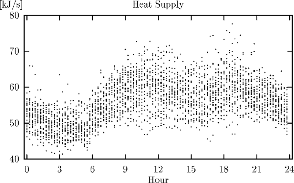
It is assumed that the heat supply can be related to the time of day, and that there is no difference between the days for the considered period. Then the regression curve is a function only of the time of day, and it is this functional relationship, which will be considered.
Figure 6.6 shows the Epanechnikov curve estimate calculated for a spectrum of bandwidths. It is clear that the characteristics of the non-smoothed averages gradually disappear, when the bandwidth is increased.
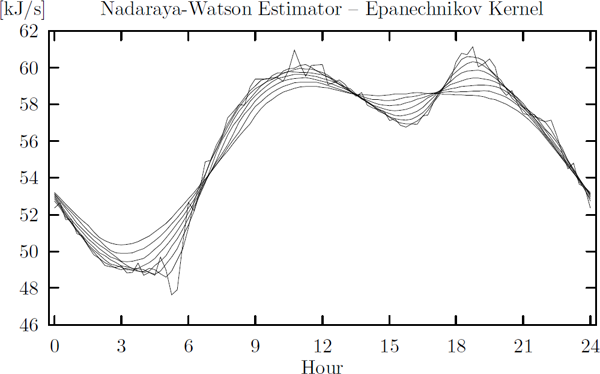
Smoothing of the diurnal power load curve using an Epanechnikov kernel and bandwidths 0.125, 0.625,..., 3.625.
When the cross-validation function is brought into action for bandwidth selection on the original data we get the result shown in Figure 6.7. Obviously the minimum of the CV-function is obtained for a bandwidth close to 1.3.
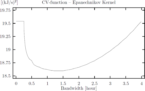
CV-function applied on the original district heating data (Kulladal/Malmö) using the Epanechnikov kernel.
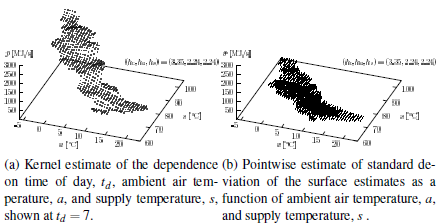
6.4.3 Non-parametric estimation of dependence on external variables — an example
This example illustrates the use of kernel estimators for exploring the (static) dependence on external variables. Data were collected in the district heating system in Esbjerg, Denmark, during the period August 14 to December 10, 1989.
The interest in this example is the heat load in a district heating system, when the two most influential explanatory variables in district heating systems, i.e., ambient air temperature and supply temperature, are included in the study.
For the estimation of the regression surface the kernel method is applied using the Epanechnikov kernel (6.15). A product kernel is used, i.e., the power load estimate, p, at time t, at ambient air temperature a and, for supply, temperature s is estimated as
where Kh(u) = k(u/h). The bandwidths were chosen using a combination of Cross-Validation and visual inspection.
6.4.4 Non-parametric GARCH models
The very large number of parametric GARCH models makes model selection non-trivial (Bollerslev [2008] for a recent overview of different models). Non-parametric GARCH models were introduced by Bühlmann and McNeil [2002] as an alternative to the non-parametric models. Their model is defined as

Heat load p(t) versus ambient air temperature a(t) and supply temperature s(t) from August 14th to December 10th in Esbjerg, Denmark.
where {Zt} is an iid sequence of zero mean, unit variance random variables. Their basic idea is to start from a parametric GARCH model, and iteratively improve the estimate of the volatility function. Their algorithm is given by:
- Estimate a simple GARCH model, recovering an approximation of the volatility {σt,0: 1 ≤ t ≤n}.
- Regress against Xt−T and to estimate the unknown function f(·,·), denoted , for m = 1,...M.
- Calculate from the estimated function .
The algorithm iterates between step 2 and 3 until the estimated function has converged.
The method was evaluated in a simulation, where the volatility is given by
It was shown in Bühlmann and McNeil [2002] that the algorithm typically converges in just a few iterations, but they also argue that it can be worthwhile to iterate a few extra times, and use the average over the estimated volatility surfaces as the final volatility forecast.
The non-parametric GARCH model was successfully used to forecast crude oil price return volatility in Hou and Suardi [2012]. This is an excellent application of the model, as the price dynamics of many commodities often are more complex than those of, say, equities.
6.5 Notes
The reader is encouraged to dig into Härdle [1990] for a more complete overview of non-parametric methods and Robinson [1983] for details on how this can be applied to dependent data.
Alternatively, semiparametric methods are nowadays an options (Ruppert et al. [2003]). The explanatory properties of semiparametric methods are similar to non-parametric methods (Härdle [2004], Hastie et al. [2009]), but there are times when these are easier to apply to data.