Chapter 4
Linear time series models
4.1 Introduction
In this chapter we introduce the concepts of linear stochastic processes and linear time series models. The description is rather condensed and far from complete. The justification for the non-completeness is that a lot of other books deal with the subjects, while the main motivation for including this chapter is for references as well as for a brief overview. For a more detailed treatment of linear time series models we refer to Box and Jenkins [1976], Brockwell and Davis [1991], Shumway [1988] and Madsen [2007].
Most of the attention is devoted to an introduction of linear time series models and a discussion of their characteristics and limitations. However, since the prediction concept is of high interest in finance, the use of linear time series models for prediction is also treated. The concept of modelling using linear time series models is only briefly mentioned.
Let us introduce some of the concepts by a very simple example.
Example 4.1 (Prediction models for wheat prices).
In this example we assume that a model is needed for prediction of the monthly prices of wheat. Let Pt denote the price of wheat at time (month) t.
The first naive guess would be to say that the price next month is the same as in this month. Hence, the predictor is
ˆPt+1|t=Pt.(4.1)
This predictor is called the naive predictor or the persistent predictor.
Next month, i.e., at time t + 1, the actual price is Pt+1. This means that the prediction error or innovation may be computed as
εt+1=Pt+1+ˆPt+1|t.(4.2)
By combining Eq. (4.1) and (4.2) we obtain the stochastic model for the wheat price
Pt=Pt−1+εt.(4.3)
If {εt} is a sequence of uncorrelated random variables (white noise), the process (4.3) is called a random walk. The random walk model is very often seen in finance and econometrics. For this model the optimal predictor is the naive predictor (4.1).
The random walk can be rewritten as
Pt=εt+εt−1+⋯(4.4)
which shows that the random walk is an integration of the noise, and that the variance of Pt is infinity, and therefore no stationary distribution exists. This is an example of a non-stationary process.
However, it may be worthwhile to try to consider a more general model
Pt=φPt−1+εt,(4.5)
called the AR(1) model (the autoregressive first-order model). A stationary distribution exists for this process when |φ| < 1. Notice that the random walk is obtained for φ = 1.
Another candidate for a model for wheat prices is
Pt=ψPt−12+εt,(4.6)
which assumes that the price this month is explained by the price in the same month last year. This seems to be a reasonable guess for a simple model, since it is well known that wheat price exhibits a seasonal variation. (The noise processes in (4.5) and (4.6) are, despite of the notation used, of course not the same.)
For wheat prices it is obvious that both the actual price and the price in the same month in the previous year might be used in a description of the expected price next month. Such a model is obtained if we assume that the innovation εt in model (4.5) shows an annual variation, i.e., the combined model is
(Pt−φPt−1)−ψ(Pt−12−φPt−13)=εt.(4.7)
Models like (4.6) and (4.7) are called seasonal models, and they are used very often in econometrics.
Notice, that for ψ = 0, we obtain the AR(1) model (4.5), while for φ = 0 the most simple seasonal model in (4.6) is obtained.
By introducing the back shift operator B by
BkPt=Pt−k(4.8)
the models can be written in a more compact form. The AR(1) model can be written as (1 − φ B)Pt = εt, and the seasonal model in (4.7) as
(1−φB)(1−ϕB12)Pt=εt.(4.9)
If we furthermore introduce the difference operator
∇=(1−B)(4.10)
then the random walk can be written ∇Pt = εt.
It is possible for a given time series of observed monthly wheat prices, P1, P2,..., PT to identify the structure of the model and to estimate parameters in that model.
The model identification is most often based on the estimated autocovariance function, since, as it will be shown later in this chapter, the autocovariance function fulfils the same difference equation as the model.
The models considered in the example above will be generalized in Section 4.4. These processes all belong to the more general class of linear processes, which again is highly related to the theory of linear systems. Therefore linear systems and processes are briefly introduced in Section 4.2 and Section 4.3, respectively. The autocovariance function is considered in Section 4.5, and, finally, the use of the linear stochastic models for prediction is treated in Section 4.6.
4.2 Linear systems in the time domain
The definition of linear stochastic processes is highly related to the theory of linear systems (Lindgren [2012]). Therefore the most important theory for linear systems will be briefly reviewed.
The following functions are needed.
Definition 4.1 (Impulse functions).
(Continuous time) Dirac's delta function (or impulse function) δ(t) is defined by
∫∞−∞f(t)δ(t−t0)dt=f(t0).(4.11)
(Discrete time) Kronecker's delta sequence (or impulse function) is
δk={1for k=00for k=±1,±2,⋯ .(4.12)
The following theorem is fundamental for the theory of linear dynamic systems.
Theorem 4.1 (Existence of impulse response functions).
For a linear, time-invariant system there exists a function h such that the output is obtained as the convolution integral
y(t)=∫∞−∞h(u)x(t−u)du(4.13)
in continuous time, or the convolution sum
y(t)=∞∑k=−∞hkxt−k(4.14)
in discrete time. The weight function, h, is called the impulse response function, since the output of the system is y = h if the input is the impulse function. Sometimes the weight function is called the filter weights.
Proof. Omitted (see Madsen [2007]). □
Often the convolution operator * is used in both cases and the output is then written as y = h * x.
Theorem 4.2 (Properties of the convolution operator).
The convolution operator has the following properties:
- a) h * g = g * h (symmetric).
- b) (h * g) * f = h * (g * f) (associative).
- c) h * δ = h, where δ is the impulse function.
Proof. Left for the reader. □
Remark 4.1.
For a given (parameterized) system the impulse response function is often found most conveniently by simply putting x = δ and then calculating the response, y = h; cf. Theorem 4.2. This is illustrated in Example 4.2.
Definition 4.2 (Causality).
The system is said to be physically realizable or causal if
h(u)=0 for u<0,(4.15)
hk=0 for k<0,(4.16)
for systems in continuous and discrete time, respectively.
After introducing the impulse response function we have
Theorem 4.3 (Stability).
A sufficient condition for stability is that the impulse response function satisfy
∫∞−∞|h(u)|du<∞(4.17)
or
∞∑k=−∞|hk|<∞(4.18)
Proof. Omitted.
Example 4.2 (Calculation of hk).
Consider the linear, time-invariant system
yt−0.8yt−1=2xt−xt−1.(4.19)
The impulse response is obtained by defining the external signal x as an impulse function δ. We then see that yk = hk = 0 for k < 0. For k = 0 we get
y0=0.8y−1+2δ0−δ−1(4.20)=0.8×0+2×1−0=2(4.21)
y1=0.8y0+2δ1−δ0(4.22)=0.8×2+2×0−1=0.6(4.23)y2=0.8y1=0.48(4.24)⋮(4.25)yk=0.8k−10.6(k>0).(4.26)
Hence, the impulse response function is
which clearly represents a causal system; cf. Definition 4.2. Furthermore, the system is stable since
Theorem 4.4 (Difference and differential equations).
The difference equation
represents a linear, time-invariant system in discrete time with the input {xt} and output {yt}, where τ is an integer denoting the time-delay.
The differential equation
represents a linear, time-invariant system in continuous time. Here t is a timedelay from the input x(t) to the output y(t).
Proof. The systems are linear because the difference/differential equation is linear, and time-invariant because the coefficients and the time-delay are constant.
Linear systems are often most conveniently described by the transfer function, in the z-domain or in the s-domain for discrete time or continuous time systems, respectively.
Theorem 4.5 (Transfer function).
A linear, time-invariant system in discrete time with input {xt}, output {yt} and impulse function {hk} is described in the z-domain by
where is the transfer function. Here Y(z) and X(z) are the output and input in the z-domain, which are obtained by a z-transformation of the sequences, i.e., and .
Proof. Use the Z-transformation on .
Notice that the convolution in the time domain becomes a multiplication in the Z-domain.
For continuous time systems the corresponding relation is
where , and , i.e., the Laplace transform of the various time domain functions. Again H(s) is called the transfer function.
4.3 Linear stochastic processes
In the rest of this chapter we only consider stochastic processes in discrete time. Stochastic processes in continuous time will be considered later on.
A linear stochastic process can be considered as generated from a linear system where the input is white noise. White noise, which will be denoted {εt}, is a sequence of uncorrelated, identically distributed random variables. Discrete time white noise is therefore sometimes referred to as a completely uncorrelated process or a pure random process. We assume in the following that the mean of the white noise process is zero and the variance is .
Definition 4.3 (The linear process).
A (general) linear process {Yt} is a process which can be written as
where {εt} is white noise, and μ is the mean of the process. (However, if the process is non-stationary then μ has no specific meaning except as a reference point for the level of the process.)
By introducing the linear operator (see Madsen [2007])
then (4.31) can be written as
Due to the close relation to linear systems Ψ(B) is called the transfer function for the process (Madsen [2007], Box and Jenkins [1976] and Lindgren [2012]).
Theorem 4.6 (Stationarity for linear processes).
The linear process given by (4.33) is stationary if the sum
converges for |z| < 1.
Proof. Omitted.
Notice the relation between stability of a linear system and Theorem 4.6.
Remark 4.2 (Cointegration).
If a time series Xt shows a linear trend and Zt = (1 − B)Xt = ∇Xt is stationary, then Xt is said to be an integrated process of order 1, which we write Xt ∈ I(1). If a time series Xt shows a quadratic trend and Zt = ∇2Xt is stationary, then Xt is said to be integrated of order 2, which similarly is written as Xt ∈ I(2).
In econometrics, additional variables are often introduced to model and, eventually, predict the variations in the process Xt. Consider the case when Xt is an I(1) process and an additional variable Yt is also an I(1) process. These are said to be cointegrated if Xt − αYt is stationary and process (Xt − αYt) is I(0) (see e.g. Johansen [1995] for an introduction to cointegration analysis).
Consider the data in Figure 4.1. It is clearly seen that the money series should be differenced once to obtain stationarity. This also pertains to the bond rate, although it is less clear. By comparing the plots to the left, it is seen that the money demand decreases when the bond rate increases and vice versa. Thus it is to be expected that these series are cointegrated.
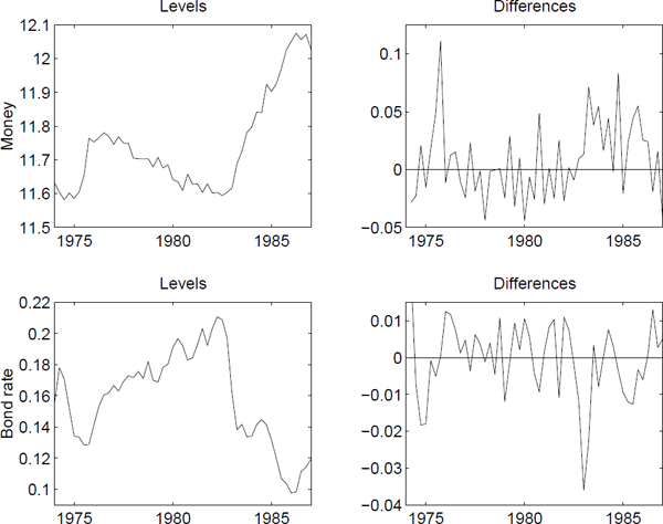
The upper-left plot shows observations from 1974:1 to 1987:3 of log real money (m2), where the log transformation has been applied to stabilize the variance. The upper-right plot shows the differenced series. The lower-left plot shows observations from the same time period of the bond rate, and the lower-right plot shows the differenced series.
4.4 Linear processes with a rational transfer function
A very useful class of linear processes consists of those which have a rational transfer function, i.e., where Ψ(z) is a rational function.
4.4.1 ARMA process
The most important process is probably the AutoRegressive-MovingAverage (ARMA) process.
Definition 4.4 (ARMA(p, q) process).
The process {Yt} defined by
where {εt} is white noise, is called an ARMA(p, q)-process.
By introducing the following polynomials in B
the ARMA process can be written as
The ARMA(p,q) process is stationary if all the roots of φ(z−1) = 0 lie inside the unit circle, and it is said to be invertible if all the roots of 0(z−1) = 0 lie inside the unit circle.
4.4.2 ARIMA process
As mentioned in the introductory example the random walk given by (1 − B)Yt = εt is a non-stationary process, since it is an integration of the white noise input.
The AutoRegressive-Integrated-MovingAverage (ARIMA) process is very useful for describing some non-stationary behaviours like stochastic trends.
Definition 4.5 (ARIMA(p, d, q) process).
The process {Yt} is called an ARIMA(p, d, q)-process, if it can be written in the form
where {εt} is white noise, φ(B) and θ(B) are polynomials of the order p and q, respectively, and both polymials have all the roots inside the unit circle.
It is clear from the definition that the process
is a stationary and invertible ARMA(p,q) process.
4.4.3 Seasonal models
As a suggestion for a very simple model for the monthly wheat prices in the introductory example we proposed to use the wheat price one year before as an explanatory variable. Assume that the seasonal period is s, then this type of seasonality can be introduced into the ARIMA model by making it multiplicative, as also illustrated in Eq. (4.9) in the case of the wheat price.
Definition 4.6 (The multiplicative (p, d, q) × (P, D, Q)s model).
The process {Yt} is said to follow a multiplicative (p, d, q) × (P, D, Q)s seasonal model if
where {εt} is white noise, and φ and θ are polynomials of order p and q, respectively. Furthermore, φ and Θ are polynomials in Bs defined by
and the seasonal difference operator is
The roots of all the polynomials (φ, θ, ϕ, Θ) are all inside the unit circle.
Example 4.3.
The number of new cars sold on a monthly basis in Denmark during the period 1955–1984 was investigated in Milhøj [1994]. The variance turned out to depend on the number of sold cars. Therefore, in order to stabilize the variance, the chosen dependent variable is
By considering, for instance, the autocovariance function, Milhφj [1994] found that the following (0,1,1) × (0, 1, 1)12 seasonal model
gave the best description of the observations.
4.5 Autocovariance functions
In this section it is assumed that the considered processes are stationary - and for simplicity it will also be assumed that the means of the involved processes are zero.
Definition 4.7 (Autocovariance function).
The autocovariance function for the stationary process Yt is
where the assumption about zero mean for Yt is used in the last equality. In order to indicate to which process the autocovariance function belongs we shall often use an index, as for instance ϒYY (k),for the autocovariance function for {Yt}.
Definition 4.8 (Cross-covariance function).
The cross-covariance function between two stationary processes Xt and Yt is
The corresponding autocorrelation function ρ(k) and crosscorrelation function ρXY(k) are found by normalizing the covariance functions using the appropriate variances, i.e.,
For a more thorough treatment of the covariance and correlation functions we refer to Madsen [2007].
4.5.1 Autocovariance function for ARMA processes
Consider the ARMA(p, q)-process:
Remark 4.3.
Notice that by multiplying the relevant polynomials the above formulation also contains the (stationary) seasonal models.
Theorem 4.7 (Difference equation for ϒ(k)).
The autocovariance function ϒ(k) for the ARMA-process in (4.50) satisfies the following inhomogeneous difference equation
where ϒεY is the cross-covariance function between εt and Yt.
Proof. Multiply by Yt−k and take expectations on both sides of (4.50).
It is noticed that for p < q
i.e., the entire autocovariance function fulfils a homogeneous difference equation.
In general it is seen that from lag k = max(0, q + 1 − p) the autocovariance function will fulfil the homogeneous difference equation in (4.52).
Remark 4.4.
Since the process is stationary all the roots of the characteristic equation corresponding to the difference equation for the autocovariance function are inside the unit circle. This means that the autocovariance (and the autocorrelation) function from lag k = max(0, q + 1 − p) consists of a linear combination of damped exponential and harmonic functions.
4.6 Prediction in linear processes
Assume that an estimate of Yt+k(k < 0) is wanted given the observations available at time t, namely Yt, Yt−1, .... The best estimate is then given by the conditional mean. We have the following fundamental result.
Theorem 4.8 (Optimal prediction).
Assume that the conditional distribution of Yt+k given the information set (Yt, Yt−1, ...) is symmetric around the conditional mean m and nonincreasing for arguments larger than m. Let the loss function be symmetric and nondecreasing for positive arguments. Then the optimal estimate is given by the conditional mean
Proof. Omitted. See for instance Madsen [2007].
Consider now, as an example, the ARIMA(p, d, q)-process
where {εt} is white noise with the variance σ2. All what follows can easily be extended to, for instance, the seasonal ARIMA model.
By introducing φ(B) = φ(B)∇d the ARIMA-process is written
where the coefficients φ1,..., φp+d are found from the identity (4.54).
If the k-step ahead forecast is wanted, we consider the equation
and simply take the conditional expectations (as prescribed by Theorem 4.8), i.e.,
In the evaluation of (4.57) we use that
Previously we have seen that the autocovariance function fulfils a homogeneous difference equation determined by the autogressive part of the model. Exactly the same holds for the predictor Yt+k|t.
Theorem 4.9 (Difference equation for optimal predictor).
For the ARIMA(p, d, q)-process (4.54) the optimal predictor satisfies the homogeneous difference equation
for k < q.
Proof. Assume that we have observations until time t, write the ARIMA-process for Yt+k, and take the expectations conditional on observations until time t. Doing this the MA-part of the model will vanish.
This is illustrated in the following example
Example 4.4 (Prediction in the ARIMA(0, d, q)-process).
Consider the ARIMA(0, d, q)-process
For k < q we obtain the homogeneous difference equation for the predictor
The characteristic equation for the difference equation has a d-double root in one. This means that the general solution is
where the superscript t on the coefficients indicates that the particular solution is found using the information set, Yt, Yt−1, ... at time t. That is, the predictor is a polynomial of degree d − 1.
4.7 Problems
Problem 4.1
Consider the linear, time-invariant system
where it is assumed that yk = 0 and xk = 0 for k < 0.
- 1. Determine the impulse response function hk for k = 0,..., 6.
- 2. Is the system stable?
Problem 4.2
Consider the first-order autoregressive process
where |φ| < 1 and {εk} is zero mean white noise with variance .
- 1. Determine the mean of yk.
- 2. Determine the variance of yk.
3. Determine the autocovariance function for (4.62).
Now assume that bond prices may be described by the ARI(1,2) process
- 4. To which order is yk defined when (4.63) is integrated?
Problem 4.3
Consider the linear, time-invariant system
where it is assumed that yt = 0 and xt = 0 for t < 0.
- Determine the impulse response function ht for t ≥ 0.
- Is the system stable?
Problem 4.4
Consider the linear system
where φ(B) = (0.8B)(1 + 7.7B) and θ(B) = (4 − B)(2 − B). It is assumed that yt = 0 and xt = 0 for t < 0.
- 1. Determine the impulse response function ht for t > 0.
2. Is the system stable?
Now consider the linear stochastic process
where {εt} is zero mean white noise with variance .
- 3. What is this process called? Is it stationary and/or invertible?
- 4. Determine and solve the difference equation for the optimal predictor for k > 2.
Problem 4.5
1. Calculate the autocorrelation for an AR(2)-process
where {εt} is zero mean white noise with variance .
2. Calculate the autocorrelation for a MA(2)-process
3. Calculate the autocorrelation for an ARMA(1, 1)-process
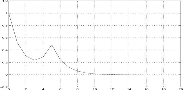
4. Determine a suitable model using the sample autocorrelogram below:
- 5. Guesstimate the parameter values (and model order) from the autocorrelation figure.
6. It is common in technical analysis when trying to predict trends to filter data using a short-length MA-filter (say an MA(5)) and a long-range MA filter (say an MA(50)). Trading strategies are subsequently triggered when these processes cross.
What are people relying on these technical analysis tools really doing in terms of linear filters?