Chapter 2

Fundamentals

A first-time home buyer is typically not able to pay the price of the new home up front, but will have to borrow against future income using the house as collateral. A company which sees a profitable investment opportunity may not have sufficient funds to launch the project (buy new machines, hire employees) and will seek to raise capital by issuing stocks and/or borrowing money from a bank. The home buyer and the company are both in need of money to invest now and are confident that they will earn enough in the future to pay back loans that they might receive.

Conversely, a pension fund receives payments from members and promises to pay a certain pension once their members retire. Insurance companies receive premiums on insurance contracts and deliver a promise of future payments in the case of property damage or other unpleasant events which people are willing to insure themselves against. The pension fund and the insurance company are both looking for profitable ways of placing current income in a way which provides income in the future.

Either way, a key role of financial markets is to find efficient ways of connecting the demand for capital with the supply of capital. The above examples should illustrate the desire of various economic agents to substitute income intertemporally (between now and some time in the future). Thus the chief mechanism by which the markets allocate capital is determined through prices. Prices govern the flow of capital.

The example on page 4 showed that interest rates play a fundamental role in the valuation of financial derivatives as interest rates are used to determine the present value of transactions, which will take place in the future, or the future value of some investments made today.

Even though the concept of interest rates is familiar to most people, the interest rate is not generally directly observable in the financial markets. Short term interest rates are quoted on a daily basis in the money markets for maturities up to approximately one year, but longer term interest rates are traded only indirectly through the bond market.

However, a lot of concepts need to be clarified before delving into this fundamental relationship between interest and (bond) prices from both a theoretical and practical point of view, but we will get back to that in later chapters.

2.1 Interest rates

Basically, an interest rate is the payment that the borrower (debtor) pays to the lender (creditor) at the end of each term for the right to use an amount that rightfully belongs to the lender.

A term is some time interval measured in days, months or years. The terms are numbered as shown in Figure 2.1. Usually transactions between the borrower and the lender are only made at the predetermined terms.

The rate of interest of one unit of account (e.g., 1 DKK) is called the interest rate, and it will henceforth be denoted by r. If r = 0.06, the borrower should pay the lender 0.06 unit of account at the end of the term per borrowed unit of account. Informally, the interest rate is the price of money.

In the following, we will assume that i) the interest rate r is deterministic and constant, ii) the number of terms n is a positive integer, iii) the interest rate is added to the capital instead of paid out at the end of the term and iv) the compounded interest is treated as the original amount.

2.1.1 Future and present value of a single payment

Assume that an initial capital c0 is deposited in a bank account with the interest rate r in n terms. It is fairly obvious that the future value of this account is

$c_n=c_0{(1+r)}^n.(2.1)$

Example 2.1 (Savings account).

Assume that a student deposits 1000 DKK in a savings account with the annual interest rate r = 0.12. Assuming that there are no taxes, this amounts to in 10 years' time

$1000\cdot {(1+0.06)}^{10}=1790.85DKK.$

Assuming that the semiannual interest rate is r = 0.03, we get

$1000\cdot {(1.03)}^{20}=1806.11DKK.$

Notice the difference between these two results, which is due to the fact that the annual rate is not just twice the semiannual rate. For a semiannual rate of 3% the annual rate will be

$({(1.03)}^2-1)\cdot 11\%=6.09\%.$

Please refer to Section 2.3 for a further discussion.

Assume that we are promised cn unit of accounts at time n. The present value or discounted value of this amount at time 0 is

$c_0=c_n{(1+r)}^{-n}.(2.2)$

The factor (1 + r)−1 is called the discount factor.

Example 2.2

Assume that you are promised 50000 DKK in 2 years' time and that the annual rate is r = 0.06. The present value is

$50000\cdot {(1+0.06)}^{-2}=44499.82DKK.$

2.1.2 Annuities

An annuity is defined as a series of equal payments that are due at some equidistant payment dates. Each payment consists of a principal and an interest. The principal accounts for the actual loan, whereas the interest accounts for the expenses associated with the loan. As we shall see in the following, Danish Government bonds and house loans, etc., are examples of annuities.

Consider an annuity with n terms. The duration of an annuity is the time elapsed from the time the loan contract has been negotiated to the last payment has been made (the n'th term). The first payments consist mainly of the principal, whereas the last payments consist mostly of the interest. Do note that the n payments are equal, but the distribution between principal and interest varies with time. The first payment of unit of account is made at the end of the first term.

2.1.3 Future value of an annuity

In the following, we will need the well-known result.

Proposition 2.1 (Finite geometric series).

The sum of a finite geometric series in q is

${\displaystyle \sum _{i-0}^{n-1}{q}^i=1+q^1+q^2+...+q^{(n-1)}=\{\begin{array}{cc}\frac{1-q^n}{1-q}& ifq\ne 1\\ n& ifq=1.\end{array}(2.3)}$

Proof. By direct calculation, we get for q ≠ 1

${\displaystyle \sum _{i=0}^{n-1}{q}^i={\displaystyle \sum _{i=0}^{n-1}{q}^i\frac{1-q}{1-q}=\frac{1-q^n}{1-q}}}$

where we used that the terms in the telescopic sum cancel out. Computing the sum when q = 1 is simply adding n terms.

Theorem 2.1 (Future value of a unit annuity).

The future value of a unit annuity as specified above is given by

$s_{n|r}\{\begin{array}{cc}\frac{{(1+r)}^n-1}{r}& ifr\ne 0\\ n& ifr=0.\end{array}(2.4)$

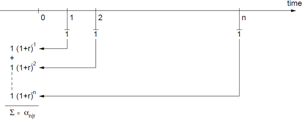
Proof. By referring to Figure 2.2, where all payments are transferred to time n using the interest rate r, we get

$\begin{array}{ccc}{c}_n& =& s_{n|r}=1+1(1+r)+1(1+r{)}^2+...+1(1+r{)}^{n-1}\\ & =& \{\begin{array}{cc}\frac{{(1+r)}^n-1}{(1+r)-1}& ifr\ne 0\\ n\hfill & ifr=0\end{array}(2.5)\hfill \end{array}$

where we have used Equation (2.3).

Corollary 2.1 (Future value of an annuity).

The future value of an annuity with equal payments c per term is

$c_n=c{s}_{n|r.}(2.6)$

Proof. Follows readily from (2.5) by replacing the unit payments by payments of amount c.

2.1.4 Present value of a unit annuity

Let us again consider an annuity with unit of account payments with a duration of n terms and a constant interest rate r.

Theorem 2.2 (Present value of a unit annuity).

The present value of an annuity as specified above is

where αn|r is called the annuity discount factor.

Proof. By referring to Figure 2.3, where all the payments are transferred to time 0, we get

$\begin{array}{lll}{c}_0={\alpha }_{n|r}& =& 1(1+r{)}^{-1}+1(1+r{)}^{-2}+...+1(1+r{)}^{-n}(2.8)\\ & =& (1+r{)}^{-1}\left[1+(1+r{)}^{-1}+...+{(1+r)}^{-(n-1)}\right]\\ & =& (1+r{)}^{-1}\frac{1-{(1+r)}^{-n}}{1-{(1+r)}^{-1}}r\ne 0\end{array}$

using Equation (2.3).

Corollary 2.2 (Present value of an annuity).

The present value of an annuity with equal payments of c units of account is

$c_0=c{\alpha }_{n|r\cdot }(2.9)$

Proof. Follows readily from (2.7).

Table 2.1 shows how αn|r varies with n and r, where 1/r is called the capitalization factor.

2.2 Cash flows

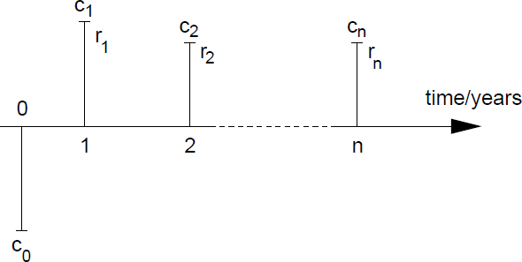
In this section we will extend the annuities (with equal payments) from the previous section to more general cash flows, where the payments at time i, i = 1,...,n, and the interest rates ri, may differ. Consider the cash flow diagram in Figure 2.4, which should be interpreted as follows: An initial investment c0 is made at time t = 0. At time t = 1, an income c1 is obtained, which should be discounted with the interest rate r1 to determine its present value, at time t = 2, the income c2 should be discounted with the interest rate r2 for two time periods, etc.

Theorem 2.3 (Present Value and Future Value).

The present value (PV) of a cash flow c = (c1,..., cn)′ discounted by the interest rates r = (r1,..., rn)′, where n is the number of time periods, is

$PV(c,r)={\displaystyle \sum _{i=1}^n\frac{c_i}{{(1+r_i)}^i}.}(2.10)$

The future value (FV) is given by

$FV(c,r)={\displaystyle \sum _{i=1}^n{c}_i.{(1+r_i)}^{n-i}.}(2.11)$

Example 2.3 (Duration).

Let FV (c, r, N) denote the (future) value of the cash flow c at time N if the interest rate is fixed at level r. Then

$\begin{array}{llll}FV(c,r,N)& =& {(1+r)}^{N}PV(c,r)& (2.12)\\ & =& {\displaystyle \sum _{i=1}^{N-1}}{c}_i{(1+r)}^{N-i}+c_N& \\ & & +{\displaystyle \sum _{i=N+1}^N}\frac{c_i}{{(1+r)}^{i-N}}.& (2.13)\end{array}$

A reasonable question to pose is how a change in the interest rate immediately after time 0 will affect FV(c, r,N). There are important effects with opposite directions which influence the risk.

1. Reinvestment risk: Assuming that r decreases, the first expression in the sum (2.13) will decrease. This decrease is caused by reinvestment risk which is due to the fact that the payments up to time N will have to be reinvested at a lower interest rate.
2. Price risk: Conversely, the last sum in (2.13) will increase when the interest rate r decreases. When the interest rate decreases the payments after time N will be discounted by a smaller factor and thus the payments will be higher. The payment af time N, cN, is unaffected by changes in the interest rate.

Theorem 2.4 (Net Present Value (NPV)).

The net present value (NPV) is given by

$NPV(c,r)={\displaystyle \sum _{i=1}^n\frac{c_i}{{(1+r)}^i}-c_0.(2.14)}$

Proof. Straightforward.

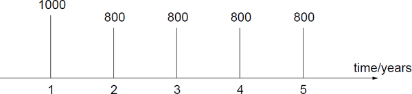
Example 2.4.

Consider the following cash flow and interest rates:

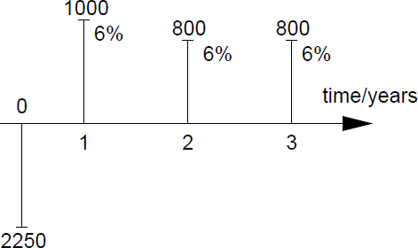
The present value is determined by (2.10);

$\begin{array}{lll}PV(c,r)& =& \frac{1000}{1.06}+\frac{800}{{(1.06)}^2}+\frac{800}{{(1.06)}^3}\\ & =& 943.40+712.00+671.70=2327.10\end{array}$

and the net present value follows from (2.14)

$NPV(c,r)=PV(c,r)-c_0=2327.10-2250.00=77.10$

Thus by investing 2250 DKK we can make a profit of 77.10 DKK measured at time t = 0.

It is an interesting problem to determine the interest rate that implies that a given cash flow has the net present value 0. This implies that the present value of, e.g., a loan is zero such that it is merely an intertemporal substitution of money.

Definition 2.1 (Internal rate of return).

The internal rate of return (IRR) y = IRR(c0, c) of a cash flow c is a solution y > −1 of the equation

$c_0={\displaystyle \sum _{i=1}^n\frac{c_i}{{(1+y)}^i}.(2.15)}$

For ci > 0, i = 0,1,..., n, the internal rate of return is called the yield.

Remark 2.1.

For a cash flow with both positive and negative future payments the IRR is not uniquely determined. In fact the polynomial (2.15) may have as many as n − 1 roots. However, IRR is uniquely determined provided that the initial payment c0 > 0 and ci > 0, i = 1, ..., n.

Remark 2.2.

Functions for determining NPV (c, r) and IRR(c0, c) for a given cash flow may be found in most spreadsheets, but can easily be computed using numerical methods (Quasi-Newton or Regula Falsi) in a general programming language.

Example 2.5 (T-maturity bullet loan).

A T-maturity bullet loan with face value F and coupon rate c is essentially described by c = (cF, cF,..., (1 + c)F)′.

Assuming that the price of a bullet loan is given by π = c0, we will show later that the internal rate of return y is not a reasonable choice of a discounting factor. It is unreasonable to assume that the interest rate will remain constant during the entire duration of the bond. The variation of the bond prices as a function of T is called the term structure of interest rates,1 and this subject will be studied in detail in later chapters. A primary goal will be to determine the interest rates r given an interest rate model and one (or possibly several) time series of bond prices.

Note that an internal rate of return is defined without referring to the underlying term structure. The internal rate of return describes the level of a flat term structure (i.e., a constant interest rate) at which the NPV of the cash flow is 0.

An application of the internal rate of return in capital budgeting is to compare some projects that one may wish to initiate in order to choose the most profitable. When this criterion is used the better project is the one with the highest IRR. Another way of choosing among alternative projects could be to compare their net present values.

2.3 Continuously compounded interest rates

As the financial markets around the world trade continuously, a more frequent quotation (than on, say, a daily basis) of interest rates is called for. Thus we will introduce continuously compounded interest rates, i.e., interest rates in continuous time, which will be used extensively in the remainder of the text.

Assume that we deposit 1 000 DKK in a bank account with an annual rate of 6%. If the interest rate is calculated at the end of the year, the bank account will contain

$FV=1000·{(1+0.06)}^1=1060 \text{DKK}$

where (2.2) have been used.

Now assume that a semiannual rate of 6%/2=3% is added twice a year

$FV=1000·{(1+0.03)}^2=1060.90 \text{DKK}.$

If a quarterly rate of 6%/4=1.5% is used, we get

$FV=1000·{(1+0.015)}^4=1061.36 \text{DKK}$

and, if we use a monthly rate of 1% each month, we get

$FV=1000·{(1+0.005)}^{12}=1061.68 \text{DKK}.$

Note that the number of interest additions during a year gives rise to a higher future value of our deposit although the annual rate remains the same.

In general, assume that the annual rate is fixed at r and that we add interest n times during a year. The future value of our deposit c0 at time 0 will in a year be

$FV=c_0{\left(1+\frac{r}{n}\right)}^n$

which readily follows from the previous computations.

It is an interesting problem to determine the compounded interest if we let the number of interest additions tend to infinity. This implies that interest is added to your account at the end of every infinitesimally small time interval during the entire year.

Theorem 2.5 (Continuously compounded interest rate).

Let n denote the number of interest additions to an account with a fixed annual interest rate r and a unit deposit at time 0. The continuously compounded interest rate is given by

Proof. Consider the function

$f(n)={\left(1+\frac{r}{n}\right)}^n=\mathit{\text{exp}} \left\{n\mathit{\text{log}} \left(1+\frac{r}{n}\right)\right\}=\mathit{\text{exp}} (g(n)).$

Introduce the change of variable $t=\frac{1}{n}$ in g(n) such that

$g\left(\frac{1}{t}\right)=\frac{\mathit{\text{log}} (1+rt)}{t}.$

A first-order Taylor expansion of log(1 + rt) yields

$\frac{rt+o(t)}{t}\to r \text{for} t\to 0^{+}.$

This implies that f(n) → er for n → ∞.

Let us illustrate the use of the continuously compounded interest rate with a couple of examples.

Example 2.6.

Assume that you deposit 1 DKK in the bank at the continuously compounded interest rate r at time 0. The future value at time t is then ert.

If you wish to use 1 DKK at time t you should deposit e−rt at time 0.

Example 2.7.

Assume that you deposit 1 DKK on a bank account with the annual rate 6%. A year later this will be worth 1.06 DKK. The corresponding continuously compounded interest rate is then

$\begin{array}{ccc}1.06=e^r& \iff & r=\text{in(1}\text{.06)=0}\text{.0586=5}\text{.86\%}\text{.}\end{array}$

This computation illustrates that one should carefully note whether it is the annual rate (a discrete time entity) or the annualized continuously compounded interest rate that is given in problems and other sources of information.

In the following we will need to be able to discount some amount C at time t = T back to time t.

Let M(t) denote the contents of a bank account with the continuously compounded interest rate r. At some time t = T, we know that the bank deposit will be C, and we need to determine its value at time t, 0 ≤ t ≤ T.

The bank deposit will exhibit exponential growth with the growth rate r

$\frac{dM}{M}=rdt(2.17)$

which has the solution

$M(t)=c{e}^{rt}(2.18)$

where c is some constant. Using that M(T) = C, we get

$M(t)=C{e}^{-r^{(T-t)}}.(2.19)$

Assuming that the continuously compounded interest rate varies deterministically with time, we get

$M(t)=C\mathit{\text{exp}} \left(-{\displaystyle \underset{t}{\overset{T}{\int }}r(s)\text{d}s}\right).(2.20)$

We will also need to be able to determine the future value of some amount using the continuously compounded interest rate. For this purpose we introduce

Definition 2.2 (Money account).

The money account process is defined by

$B(t)=exp\left({\displaystyle \underset{0}{\overset{t}{\int }}}r(s)ds\right)(2.21)$

or

$\begin{array}{llll}dB(t)& =& r(t)B(t)dt& (2.22)\\ B(0)& =& 1& (2.23)\end{array}$

where r(t) denotes the continuously compounded interest rate at time t.

The money account is simply a formal way of saying “money in the bank,” because the amount B(t) is compounded continuously with the interest rate r(t). Note, in particular, that the interest rate may be described by a stochastic process, and that we just plug in a given sample path of the interest rate in (2.21). By reverting the time in (2.21) (in which case we get (2.20)), it also serves as a simple model of bonds, such as Danish Government bonds or US Treasury bills.

2.4 Interest rate options: caps and floors

So far we have assumed interest rates to be deterministic, but this is clearly at odds with reality. Consider, e.g., the Copenhagen InterBank Offered Rate (CIBOR) in Figure 2.5, which is the interest rate banks use when they loan or borrow money from one another. These rates are quoted for a number of maturity dates, i.e., they are interest rates associated with loans on a 1, 3 or 6 months basis.

Referring to Figure 2.5, the first 600 observations (1/2 1990 to 1/7 1992) of the interest rates fluctuate around approximately 10% with slightly higher values at both ends of the period. Following this stable period, the currency turmoil begins in the fall of 1992. First, the pound drops out of the EMS (European Monetary System) on 22/9 1992 where the CIBOR 1M2 is set at 35%, whereas the CIBOR 3M and 6M equal 14.875% and 12%, respectively. In November 1992, the international currency traders turned their attention towards the Scandinavian currencies. The first attack was on the Finnish markka on 8th September, that also influenced the Norwegian and Swedish currencies. This was followed by devaluations of the Italian lire on 14th September and the Spanish peseta on 17th September and the pound dropping out of the EMS on 22th September. Attention was the redirected towards the scandinavian currencies again, with the Swedish krona floating from 19th November an attacks on the Norwegian krone peaking at 23rd November (this is the first peak in Figure 2.5). The speculation continued through the year (the second cluster of peaks in Figure 2.5) with a third cluster in 2013. These attacks are easily seen in the group of observations numbered around 700–750, i.e., November–December 1992. The first peak on the November 11, 1992 was due to an attack on the Finnish markka, the second peak concerns the Norwegian Krone December 12 and finally attention was turned to the Swedish Krona around December 11. On this date, the CIBOR 1M was raised to 34%. During this period the National Banks in the Scandinavian countries spent large amounts of money trying to defend their currencies. Later, in February 1993, the Danish Krone came under attack and the CIBOR 1M was raised to 32.75% on February 8.

Following this turmoil, the interest rates drop exponentially until the French Franc is brought into focus during July and August 1993, where the CIBOR 1M is raised to 24.7% on August 3, 1993. Although the figures in this last period do not seem to be as externally determined as the previous periods of currency turmoil, which might indicate that a very high level of volatility is present in the series/markets, it is deemed that some interventions are made by the National Banks.

By considering the three time series as a collection of three-dimensional stochastic variables, the correlation structure of the time series is easily obtained:

$\left[{\rho }_{ij}\right]=\left(\begin{array}{ccc}1.0000& 0.9356& 0.8311\\ 0.9356& 1.0000& 0.9611\\ 0.8311& 0.9611& 1.0000\end{array}\right).(2.24)$

It is readily seen that the CIBOR interest rates for different maturities are strongly correlated, although it can be seen graphically that the correlation varies (decreases) over time. More specifically, the correlation between the interest rate was stronger prior to the events described in the text above.

Although some of the large variations in the CIBOR series may be explained by interventions from the National Banks, it is clear that market participants would like to protect themselves against such large variations in the interest rates. Indeed, a large number of interest rate derivatives have been derived with this application in mind. Some of these use the interest rate itself as the underlying asset. In the following we will consider two interest rate derivatives: The cap is a contract that can be used to protect a borrower against floating or stochastic interest rates being too high. A cap can be thought of as a series of interest rate options (these are called caplets.) Conversely, a floor is a contract that can be used to protect a lender against floating interest rates being too low.

Example 2.8 (A simple interest rate option).

We will consider a 6 Month European-style Call option on the 6 Month LIBOR3 at a strike level of 8% and a face value of 10 Million USD. We will assume that this option costs 30000 USD, which corresponds to 3% of the face value (or 30 basis points of the face value).

Let us adapt a tabular form of specifying the details of the option:

This call option gives the buyer the right but not the obligation to receive the difference between the 6 Month LIBOR interest rate (the underlying) prevailing in six months' time (the expiration date) and the 8% strike level, if the former happens to be greater. Thus the buyer of such an option receives a higher payoff as interest rates rise. The face value determines the size of the contract. The payoff function is as follows:

Thus, the payoffis determined by the difference between the actual interest rate r in 6 months (expressed as an annual rate in percent) and the strike level of 8%. This is multiplied by the actual number of days in the subsequent six months period as a proportion of the 360 days in a year (!), and the face value of the option. Note that this payoff is received on the maturity date of the underlying interest rate, i.e., 183+182 =365 days from today. Thus, the current time (t = 0 days) is when the contract is written, the contract expires in 183 days and the payoff of the underlying face value will be received 365 days from today. Assuming that the actual interest rate in 183 days' time is 9%, the following payoff is obtained:

$(9\%-8\%)\cdot 182/360\cdot 10 \mathit{Million} \mathit{USD}=50555 \mathit{USD}$

and this amount will be received 365 days from today. Let us compute the break-even point, i.e., the interest rate i, where the total borrowing cost would be the same with and without the call option. This is not the strike level of 8%, because we have to take the price of the option 30 000 USD into account.

Assuming that we didn't purchase the option, the cash flow on the repayment date of the loan of $10 million on the maturity date would be

$10 million USD\cdot \left[1+(i\%\cdot 182/360)\right].$

Using the call option, the interest rate will be limited by the strike level. Thus the total payment on the loan on the maturity date would be

$10 million USD\cdot \left[1+(8\%\cdot 182/360)\right].$

Recall that the option itself costs $30000 today, and we have to compute the future cost on the maturity date. The interest rate for the first six months (183 days) is known today, but the interest rate for the second six month period (182 days) is not known today. However this was denoted by i such that the compounded cost of the option is

$30000 USD\cdot \left[1+(8\%\cdot 183/360)\right]\left[1+(i\%\cdot 182/360)\right].$

Thus the break-even point may be found from the equation

$\begin{array}{l}10 million USD\cdot \left[1+(i\%\cdot 182/360)\right]=\\ 10 millionUSD\cdot \left[1+(8\%\cdot 182/360)\right]\\ +30000 USD\cdot \left[1+\left(8\%\cdot 183/360\right)\right]\left[1+\left(i\%\cdot 182/360\right)\right].\end{array}$

By solving this with respect to i, we get

$i=8.64\%.$

This implies that the option starts to pay if the interest rate at the expiration date exceeds 8.64%. If the interest rate is lower at the expiration date, we would have been better off without the option.

An interest rate cap is a series of European call options. Let us consider an example.

Example 2.9 (Caps).

We consider a 5 year cap on 6 month LIBOR at 8% with a face value of 100 million USD

Essentially we wish to borrow 100 million USD and protect ourselves against interest rates above 8%. This protection is obtained by purchasing a cap at the cost of 3 million USD. Assume that we wish to pay this amount as a stream of periodic payments. Since the term of the cap is 5 years, there are 10 periods of 6 months involved. However, since the interest rate for the first period is known today, we need not purchase an option on this rate. Hence there are 9 options in the cap (each of these is called caplets) with payoffs to be determined on the reset dates: January 13 and July 13. The stream of periodic payments may be considered as a cash flow which should be balanced against the upfront fee of $3 million. Using a semiannual rate of 4%, we could determine the size of the 9 payments using (2.7)

$c=\frac{c_0}{{\alpha }_{n|r}}=\frac{3000000}{{\alpha }_{9|4\%}}=\frac{3000000}{\frac{{(1.04)}^9-1}{{(1.04)}^9\cdot 0.04}}=403479USD.$

Thus we should pay 403 479 USD every 6 months for the next 4.5 years. However, these payments were computed under the assumption of equal interest rates during this period. We have to consider the multiperiod scenario of the cap spanning over 4.5 years, where the interest rate will be floating or vary randomly. If this is taken into account the payoffs from the cap depend on the whole sequence of future interest rates. Again, it turns out that we need to know something about future interest rates in order to price financial derivatives. An assessment of these future rates will be based on the term structure of interest rates.

2.5 Notes

The material in this chapter is based on Lynggaard [1993], which contains a number of examples and exercises. In addition in the lecture notes, Lando [1996] provides an excellent introduction to mathematical finance in general. An excellent introduction to a wide class of financial derivatives is Figlewski et al. [1991]. In particular, this book contains a large number of carefully worked examples.

2.6 Problems

Problem 2.1

1. Show the limits in Table 2.1.

Problem 2.2

Consider an European call option on the amount Y of USD with exercise date T and strike price K.

1. Explain why a higher strike price K gives rise to a lower price Π on the option.

Problem 2.3

Consider an European call option on the amount Y of USD with exercise date T and strike price K. Let c0 denote the arbitrage-free price of this option.

1. Draw the payoff diagram.

Problem 2.4

Consider the following cash flow:

Assume that the interest rate is r = 0.12.

1. Compute the present value c0 = PV(c, r).
2. Compute the future value c5 = FV(c, r).
3. Determine the initial payment c0 for this cash flow such that the net present value is 0.

Problem 2.5

The Simpson family wish to have saved 100 000 in a bank account for a new car in 5 years.

1. Determine the monthly deposits to a bank account assuming that the monthly interest rate is r = 1%.

Problem 2.6

A man borrows 10 000 DKK at time 0 for three years, which should be paid back as an annuity loan, i.e., as n = 3 equal payments a. The annual interest rate is r = 0.06.

1. Compute the payment c per term. Each payment of equal amount consists of a payment of principal and interest. The last two differ from one-period to another.

2. Complete the following table:

   Time	Payment	Interest	Principal	Remaining debt
   0				10000
   1		600
   2
   3

Problem 2.7

Show that

$s_{n|r}^{-1}={\alpha }_{n|r}^{-1}-r.$

Problem 2.8

Consider the cash flow c = (c0, c1, c2)′. The internal rate of return y is the solution to the equation

$c_0=\frac{c_1}{1+y}+\frac{c_2}{{(1+y)}^2}(2.25)$

as stated in Definition 2.1.

1. Show that there may exist two solutions (y1, y2) such that the internal rate of return y is not uniquely specified.

Problem 2.9

Consider the following cash flow:

1. Assuming that the annual rate is 6%, what is the present value of this cash flow?

   Consider the same cash flow with different interest rates as shown below:

   

2. Determine the initial payment c0 such that the present value is 0.

   Consider the following cash flow with net present value 3600.78.

   

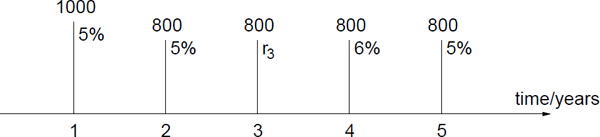
3. Determine the interest rate r3.

Problem 2.10

Assume that you deposit 1 DKK in a bank account with an annual rate of 12%.

1. Determine the continuously compounded rate r.

Problem 2.11

Consider an annuity with n terms with equal payments c, a duration of n periods and the constant interest rate r.

If the first payment is made at the end of the first term the present value is given by (2.7). Consider the more general case, where the first payment is made at term k, where 0 < k < n.

1. Plot the cash flow in a diagram similar to Figure 2.3.
2. Derive a formula for the present value in the more general case. The formula should contain α.|r.

Problem 2.12

Consider the simple market on page 4.

1. Show that the discount factor β = B0/B1 is given by

   $\beta ={(1+r)}^{-1}$

   where r is the annual rate.

2. Now assume that the price of the bond at time t = 1 is fixed at B1. Explain what will happen to the bond price at time t = 0, B0, if the interest rate r goes up or down. Plot B0 as a function of r for reasonable values of r.

Problem 2.13

1. Show that (2.20) simplifies to (2.19) for r(t) = r, i.e., a constant rate.

1A constant interest rate implies that the term structure is flat.

2CIBOR 1M is short for the one-month CIBOR time series, etc.

3LIBOR is short for London InterBank Offered Rate.