Chapter 13
Parameter estimation in discretely observed SDEs
13.1 Introduction
This chapter describes methods for estimating parameters in stochastic differential equations (SDEs). A brief introduction to the GMM method is given, but a major part of the presentation is devoted to a class of maximum likelihood methods which can be used for estimation parameters in both linear and non-linear SDEs.
It is clear that a method for estimating parameters of non-linear stochastic differential equations can also be used for estimating the parameters of a linear stochastic differential equation. If a linear model is considered, it is, however, advantageous to take the linearity into account at the estimation procedure. Likewise it is beneficial to simplify the method if it is known that the model is time invariant.
In this section we shall briefly introduce the various types of models which will be considered in the subsequent sections.
There are several reasons why it is advantageous to consider the continuous-discrete time state space approach:
- If any physical knowledge is available it is easily included in the model, since the system equation is described in continuous time.
- The estimated parameters are readily interpreted by experts in the field.
- Multivariate models are easily considered.
- Time varying models can be handled.
- Missing observations, as well as time varying sampling times, can be handled.
- It is often the case that less parameters are needed for the continuous time formulation than for the traditional discrete time formulation.
- The solution of the Itō equation is a Markov process.
The main limitation is the difficulty to derive estimators, or, rather, deriving the Maximum Likelihood estimator in closed form. Instead, we have to rely on approximations of the Maximum Likelihood estimator.
There are some perhaps unexpected results1 regarding asymptotic properties of the estimators that are useful to know.
Example 13.1 (Estimating parameters in the drift and diffusion).
Consider the arithmetic Brownian motion
dX(t)=μdt+σdW(t).(13.1)
The solution is well known, X(tn+1) − X(tn) = μ(tn+1 − tn) + σ(W(tn+1) − W (tn)), implying that each difference of observations is an independent Gaussian random variable. All that is needed is to compute the mean and covariance! The drift is estimated by computing the mean, and compensating for the sampling δ = tn+1 − tn
ˆμ=1δNN−1∑n=0X(tn+1)−X(tn). (13.2)
Expanding this expression reveals that the MLE for μ is given by
ˆμ=X(tN)−X(t0)tN−t0.(13.3)
The only thing that matters is the lengths of the observation window; recording measurements inside the sample is of no use whatsoever for the drift parameter.
The situation is different for the diffusion (σ) parameter, as the MLE is given by
ˆσ2=1δ(N−1)N−1∑n=0(X(tn+1)−X(tn)−ˆμδ)2d→σ2χ2(N−1)N−1(13.4)
which converges to the correct quantity. The σ parameter can be well estimated by either having a short sampling interval and sampling frequently, or by having a fixed sampling frequency and sampling for a very long time.
13.2 High frequency methods
It should be clear from Example 13.1 that the variance term can be estimated using high frequency data. In fact, that variance estimator is closely linked to the convergence of the stochastic integral and the Itō formula. Here we assume that the process we study is a compound Poission Jump Diffusion
dX(t)=μ(t,X(t))dt+σ(t,X(t))dW(t)+dZ(t)(13.5)
with Z(t)=ΣN(t)n=1Jn where J are the stochastic jumps and N(t) is the Poisson process.
Let πN = [0 = τ0 < τ1 < ... τN = T] be a partition of the interval [0, T], where sup |τm+1 − τm| 4 0, and define
RV=N∑n=1(X(τn)−X(τn−1))2.(13.6)
Then it follows the statistic RV, called the Realized Variance estimator, converges to the Quadratic Variation (QV) of the process, cf. Section 13.7.
RVp→∫σ(s,X(s))2ds+N(t)∑n=1J2n=QV(13.7)
while a small modification called the bipower estimator defined as
BPV=π2N∑n=1|X(τn+1)−X(τn)||X(τn)−X(τn−1)|(13.8)
converges to the continuous component
BPVp→∫σ(s,X(s))2ds.(13.9)
Shifting the computations a single step will eliminate jumps as the jumps only contribute to one of the terms, while the other term will be very small when the partitioning gets finer and finer.
The implication of these methods (Barndorff-Nielsen [2002], Barndorff-Nielsen and Shephard [2004]) is that high frequency data can be used to estimate the variance and jump parts with very good accuracy. However, market microstructure (Hansen and Lunde [2006], Zhang et al. [2005]), generally prevents us from going to the limit, and there seems to be a consensus that sampling too often will contaminate the data more than the additional variance reduction obtained due to the larger data set.
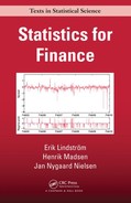
We illustrate the realized volatility by computing it on simulated data from a geometric Brownian motion; see Figure 13.1. The constant volatility of the log returns implies that the integrated squared volatility grows linearly.

Computing the realized variance and bipower variation on index returns on the Swedish 0MXS30, as shown in top graph in Figure 13.2, reveals that the variance is not constant; cf. Section 5.5.2 and 5.5.3.
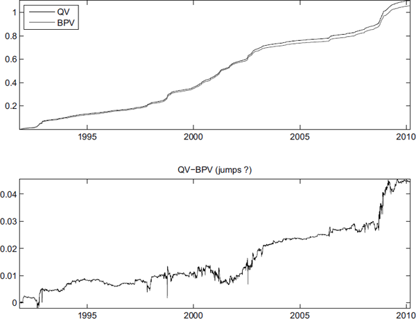
Realized variance and bipower variation computed on log returns on the OMXS30 index (top graph) and the difference between the bipower variation and realized variance (bottom graph).
These statistics can also be used to investigate whether there are jumps as the difference RV − BPV should equal to the sum of the squared jumps
RV−BPVp→N(t)∑n=1Jn.(13.10)
This difference is computed in the lower graph in Figure 13.2, where some evidence for jumps is presented. Notice that most jumps are rather modest in size, and also that the jumps often seem to cluster to periods of high variance.
Realized volatility was used in Phillips and Yu [2009] to derive Maximum Likelihood estimators for some diffusion processes by first estimating the integrated volatility and then using methods like those in Section 8.4.4.
13.3 Approximate methods for linear and non-linear models
The complexity estimating parameters in discretely observed diffusions, i.e., estimating parameters when the full state vector is observed as discrete time points, depends on a number of factors, most important being the dynamics of the process and the sampling frequency.
Many data sets are sampled at high frequency, compared to the dominant dynamics of the stochastic system, making the bias due to discretization of the SDEs using any of the schemes in Chapter 12 acceptable.
The simplest discretization, the explicit Euler method, would for the stochastic differential equation
dX(t)=μ(t,X(t))dt+σ(t,X(t))dW(t)(13.11)
correspond to the Discretized Maximum Likelihood (DML) estimator given by
ˆθDML=argmaxθεΘN−1∑n=1log ϕ(X(tn+1),X(tn)+μ(tn,X(tn))Δ,∑(tn,X(tn))Δ)(13.12)
where ϕ (x, m, P) is the density for a multivariate normal distribution with argument x, mean m and covariance P and
∑(t,X(t))=σ(t,X(t))σ(t,X(t))T,(13.13)
and Δ = tn+1 −tn is the time between two consecutive observations.
Note that the Euler scheme and the Milstein scheme coincide when the diffusion term is independent of the state vector. Similarly, it was shown in Chapter 12 that higher order method can readily be derived when the diffusion term is independent of the state vector, which indicates that transformations to get rid of state dependence are generally a good idea.
13.4 State dependent diffusion term
If the SDE contains a state dependent diffusion term then the methods described in the previous section cannot be used directly. Frequently it is, however, possible to transform the SDE into an equivalent SDE where the diffusion term is independent of the state vector. The equivalent SDE contains the same parameters and describes a relation between the same input and output variables.
13.4.1 A transformation approach
We shall only consider the scalar case here. The transformation approach is based on the Itō formula which we restate here for convenience.
Theorem 13.1 (The Itō formula).
dX(t)=μ(t,X(t))dt+σ(t,X(t))dW(t)(13.14)
and φ: ℝ2 ↦ ℝ be a C1,2(ℝ2)-function applied toX(t)
Y(t)=φ(t,X(t)).(13.15)
Then it holds that
dY(t)=[∂φ∂t+μ∂φ∂X(t)+12σ2∂2φ∂X(t)2]dt+g∂φ∂X(t)dW(t).(13.16)
Proof. See page 147.
Notice that the diffusion term in the new Itō process dY(t) is equal to the product of g and ∂φ/∂x. This leads us to the following lemma.
Lemma 13.1.
Let X(t) and φ be defined as above, then by choosing the transformation
ϕ(xt,t)=∫1σ(t,X(t))dX(t)(13.17)
the new process Z(t) = φ(X(t),t) will be an Itō process with a constant diffusion term.
The procedure is easily generalized to the multivariate case where the matrix g(X(t),t) only contains non-zero values on the diagonal, but is far more complicated in the general case (cf. Aït-Sahalia [2008]).
Example 13.2 (Transformation of the CKLS-model).
Consider the CKLS-model (Chan et al. [1992]):
dX(t)=α(θ−X(t))dt+σX(t)γdW(t)(13.18)
where X(t) is the short term interest rate, and α and θ are parameters related to the drift term and δ and γ are related to the diffusion term.
The drift term represents a tendency to pull the process back towards its long-term mean θ with the rate of adjustment determined by α. The diffusion term describes that the variability (the volatility) is increasing with x if γ > 0.
Some important models used in the field of finance are obtained as a special case of the CKLS-model:
γ=0 we get the Vasicek model (Vasicek [1977])γ=12 we get the Cox−Ingersoll−Ross model (Cox etal. [1985])
By applying the lemma, the following transformation is suggested in order to obtain a constant diffusion term in a new process which contains the same parameters and relates the same input and output.
Z(t)=φ(xt,t)=∫1X(t)γdX(t)=11−γX(t)1−γ.(13.19)
The SDE for Z(t) is found by using the Itō formula. Hence we need
∂φ∂t=0,∂φ∂x=X(t)−γ,∂2φ∂x2=−γX(t)−y−1.(13.20)
Insertion into the Itō formula leads to the following SDE for Z(t)
dZ(t)=[αθ((1−γ)Z(t))γγ−1−α(1−γ)Z(t)−γσ22(1−γ)Z(t)]dt(13.21)+σdW(t)(13.22)
13.5 MLE for non-linear diffusions
It is rarely possible to do full maximum likelihood estimation for non-linear diffusions, but the likelihood function can often be approximated arbitrarily well. Some technical difficulties are avoided if the class of models is restricted to discretely observable models.
There are at least three types of competing algorithms that are computationally efficient. The most general, and also the computationally least efficient class of algorithms, are the Monte Carlo simulation based estimators. The Fokker-Planck based estimators are computationally more efficient (at least in low dimensions). Finally, the series expansion approach is the computationally most efficient algorithm but it is also the most restrictive estimator. Common for all estimators is that their computational efficiency is usually improved if the diffusion term is independent of the states of the process; cf. Section 13.4.
13.5.1 Simulation-based estimators
The class of simulation based estimators can be applied to virtually any continuous time Markov process, for which a numerical scheme has been derived. The basic idea is to calculate the unknown transition probability density p(xt|xs) by successive approximations. Assume that s < τ1 < τi < τN − 1 < t. The transition probability density is then (due to the law of total probability and the Markov property) given by
p(xt|xs)=∫p(xt|xτi)p(xτi|xs)dxτi.
This can be iterated N times, and the following expression is derived
p(xt|xs)=∫p(xt|xτN)∫⋯∫p(xτ1|xs)dxτ1...dxτN.
The N × dX dimensional integral (dX = dim(X(t))) is easily calculated using Monte Carlo methods (e.g. Pedersen [1995]). An implementation of this algorithm is actually quite easy as the numerical representation of the integral
p(xt|xs)=∫p(xt|xτ)p(xτ|xs)dxτi
is given by
pK(xt|xs)=1KK∑k=1p(xt|xkτ)
where xkτ was generated from p(xτ|xs), see Chapter 12 for numerical schemes. However, the simple Monte Carlo approximation is usually too inaccurate to be useful (e.g. Durham and Gallant [2002]), and variance reduction is regularly applied. An efficient version was introduced in Durham and Gallant [2002], and uses a combination of antithetic variables, moment matching and importance sampling (so-called Brownian bridge sampler, see Problem 8.9). Lindström [2012a] improves that Brownian bridge sampler further by introducing a regularization term that improves the performance for sparsely sampled models.
The simulation based estimators converge as 1/√K regardless of dimension. This leads to relatively slow convergence in low dimensions but is very competitive in higher dimensions.
13.5.1.1 Jump diffusions
Similar methods have been developed for jump diffusions and Lévy driven SDEs (e.g. Hellquist et al. [2010], Lindström [2012b]). A computationally attractive alternative to direct maximization of the likelihood function is to use the EM algorithm (e.g. Sundberg [1974], Dempster et al. [1977]).
The EM algorithm finds the Maximum Likelihood estimate by iteratively alternating between computing the Expectation of the intermediate quantity
Q(θ,θ′)=E[log pθ(X,Y)|Y,θ′](13.23)
where X are some latent variable and Y the observations, and maximizing that quantity
θm+1=argmax Q(θ,θm).(13.24)
Computing the posterior distribution is similar to the simulated maximum likelihood methods. Define Y as the observations (Y = Yt1,...,YtN) and X = (Xτ1,..., XτN−1) as latent values of the process in between the observation (t1 < τ1 < ... < τN−1 < tN). The posterior is then given by
p(Xτn|Ytn,Ytn+1)∝p(Ytn+1|Xτn)p(Xτn|Ytn).(13.25)
It is therefore possible (this is very similar to what is done in the bootstrap filter, see Section 14.10) to use resampling of particles generated from the naive dynamics to compute a sample from the posterior distribution (Lindström [2012b]).
The intermediate quantity will typically be easy to maximize as the transition density for a short time interval is well approximate using even simple discretization schemes (cf. Chapter 12), typically leading to a sum of logarithms of Gaussian densities.
13.5.2 Numerical methods for the Fokker-Planck equation
The Fokker-Planck based estimators apply deterministic numerical schemes to the Fokker-Planck equation, a parabolic partial differential equation governing the evoluation of the transition probability density.
The Crank-Nicholson scheme was applied in Lo [1988] while Lindström [2007] used higher order schemes as well. It is usually computationally efficient to use higher order finite difference schemes. The Fokker-Planck equation is typically solved by defining a grid in the domain of the process and approximating the derivatives in the domain with central differences on the grid. This reduces the partial differential equation
∂p∂t(x,t)=−∂∂x(μ(xt)p(x,t))+12∂2∂x2(σ2(xt)p(x,t))
to a system of linear differential equations
dpdt(t)=Ap(t)+b
which has a closed form solution. It was shown in Lindström [2007] that the rate of convergence of the Fokker-Planck based estimators is significantly faster than, i.e., simulation based estimators, but it is known the rate deteriorates as the dimension increases.
The partial differential equation approach can also be used to compute moments or eigenfunctions, which could lead to substantial computational savings as fewer PDEs need to be solved numerically. These can be used to derive GMM or Quasi-likelihood estimators (see Höö k and Lindström [2014] for details).
13.5.3 Series expansion
The Aït-Sahilia estimator (Aït-Sahalia [2002, 2003]) derives a closed form expression of the transition probability density. This is achieved by approximating the true transition probability density by a standard Gaussian random variable and correcting for the deviations using Hermite polynomials (Hermite polynomials are orthogonal polynomials associated to the standard Gaussian density). Unfortunately the correction only does converge if the true density is similar to the standard Gaussian density.
The solution in Aït-Sahalia [2002] is to transform the process dX(t) = μX (X(t))dt + σX (X(t))dW(t) to a new representation where the diffusion term is independent of X(t); cf. Section 13.4. This can be achieved by introducing
Y(t)=γ(X(t))=∫X(t)duσX(u)
resulting in
dY(t)=(μX(γ−1(Y(t)))σX(γ−1(Y(t)))−12∂σX∂x(γ−1(Y(t))))dt+dW(t).
The second step is to normalize Y(t) by its approximative standard deviation
Z(t)=Y(t)−Y(s)√t−s.
The density for Z(t) is then expanded in Hermite polynomials (orthogonal polynomials with respect to the Gaussian density) as
pZ(z|ys)=ϕ(z)(1+∞∑j=1η(j)Z(t−s,ys;θ)Hj(z)),
where the formula to calculate η(j)z=1/(j!)EZ[Hj(Z)] is given in Aït-Sahalia [2003], Hj(z) are Hermite polynomials and ϕ(z) is the density of a standard Gaussian random variable. The closed form expression for pz(z|ys) is then used to calculate pX(xt|xs). It is not guaranteed that the Hermite expansion will generate a pdf (i.e., a density that ≥ for all function values and integrates to one). Another approach is then to work with log densities (log p) rather than densities (p) (Aït-Sahalia [2002]). That would eliminate the risk for negative densities, but the approximation will still not integrate to one, unless infinitely many terms are included in the expansion.
The estimator is very efficient from a computational point of view when t − s is small. A multivariate version of the algorithm was presented in Aït-Sahalia [2008], but the generalization is not as smooth as one could hope; the expansion is only valid for so-called reducible diffusions, which excludes many models in financial economics such as stochastic volatility models.
13.6 Generalized method of moments
The Generalized Method of Moments is a method attributable to Hansen [1982] which can be used for estimating parameters in stochastic differential equations. Similar ideas (called estimation function) can be found in Bibby and Sørensen [1995]; see Sørensen [2012] for a recent overview.
For the GMM method no explicit assumption about the distribution of the observations is made, but the method can include such assumptions. In fact, it is possible to derive the ML estimator as a special case of the GMM estimator.
The standard version of the GMM method requires that all the state variables are observed directly. This is clearly a drawback of the method, since it dramatically limits the complexity of the models which can be considered. In the modeling of spot interest rates, this is a severe restriction, due to the fact that the spot interest rate is not observed directly, but only implicitly via the bond prices. Furthermore, the estimation does not take place directly in the continuous-time model; the stochastic differential equations must be discretized (see Chapter 12), before using the GMM method, and the sampling time must be constant. The best reference to discretization techniques so far is Kloeden and Platen [1995] and Platen and Bruti-Liberati [2010]; see also Chapter 12.
13.6.1 GMM and moment restrictions
We shall introduce the moment restrictions by first considering an example which is of great interest in statistical finance.
Example 13.3 (GMM estimates of the CKLS model).
Consider the following stochastic differential equation
dr(t)=(θ+ηr(t))dt+σr(t)γdW(t)(13.26)
where W(t) is a standard Wiener process. This model, which is called the CKLS model (Chan et al. [1992]), is often used to model the short term risk-less interest rate. The structure of the CKLS model implies that the conditional mean and variance of the short term rate depend on the level of r(t).
The observations are in general given in discrete time. Hence the model (13.26) has to be formulated in discrete time before setting up any moment restrictions which can be evaluated using the discrete time data.
In financial and economical applications the Euler approximation method (see Chapter 12) is most often used to formulate the discrete time equivalent of the continuous time model. Using the Euler approximation of model (13.26) we obtain the following discrete time model
rk+1=rk+(θ+ηrk)Δ+εk+1(13.27)
where
E[εk+1|Bk]=0(13.28)E[ε2k+1|ℱk]=σ2r2γkΔ(13.29)
and where ℱk denotes the information set at time tk.
Under the assumption that the restrictions implied by the model, i.e., by (13.27), (13.28) and (13.29) are true, the following moment restrictions follow
E[εt+1−E[εt+1|ℱt]]=0,(13.30)E[ε2t+1−E[ε2t+1|ℱt]]=0.(13.31)
The GMM procedure consists of replacing the expectation E[·] with its sample counterpart, using the N observations available {r(k); k = 1,...,N}.
Now we are ready to formulate the GMM method more formally. Assume that the observations are given as the following sequence of random vectors:
{xt;t=1,...,N}
and let θ denote the unknown parameters (dim(θ) = p).
Let f(xt, θ) be a q ≥ p-dimensional zero mean function, which is chosen as some moment restrictions implied by the discretized model of xt.
The GMM estimates are found by minimizing
JN(θ)(1NN∑t=1f(xt,θ))TWN(1NN∑t=1f(xt,θ)) (13.32)
where WN ∈ ℝq×q is a positive semidefinite weight matrix, which defines a metric subject to which the quadratic form has to be minimized. The key observation is that any remaining bias in the moment conditions (e.g., (13.30) or (13.31)) is going to increase the JN function.
Example 13.4 (GMM estimates of the CKLS model (cont.)).
Consider again the CKLS model given in Eq. (13.26), and the Euler approximative discrete time equivalent model given by (13.28)–(13.29). The unknown parameters are θ = (θ, η, γ, σ)T.
In order to use the GMM method we may use the moment restrictions given by
f(rk,θ)=(εk+1−E[εk+1|ℱk](εk+1−E[εk+1|ℱk])rkε2k+1−E[ε2k+1|ℱk](ε2k+1−E[ε2k+1|ℱk])rk)=(εk+1εk+1rkε2k+1−σ2r2γkΔ(ε2k+1−σ2r2γkΔ)rk).(13.33)
Note that in the second and fourth equation the variable rk is used as an instrumental variable. Those equations are justified by the fact that rk is independent of the entities (ε2t+1−E[εk+1|ℱk]) and (ε2t+1−E[ε2k+1|ℱk]).
Some extensions of the GMM for diffusions include Simulated GMM often called Simulated Method of Moments (SMM) (McFadden [1989]). Monte Carlo simulations can be used to compute arbitrarily accurate approximations of moments, thereby eliminating the bias caused by the discretization scheme. Solving PDEs is a computationally attractive alternative in many cases (Höök and Lindström [2014]).
The characteristic function is known for a fairly large class of processes, as presented in Section 7.5. These can be used to construct suitable moments without having to use any discretization scheme (Singleton [2001] and Chacko and Viceira [2003]). It can be useful to add many moment conditions (Carrasco et al. [2007]), who showed that Maximum Likelihood efficiency is achieved when a continuum of moments is employed in the estimation, although there is a practical upper limit when employing the method on real data (for example, the number of conditions has to be smaller than the number of observations).
Another approach suitable for diffusion (or Markov processes in general) is to use eigenfunctions of the generator as moments (Kessler and S⊘rensen [1999]). The downside is that these can be tricky to compute, and other methods may be preferred (i.e., maximum likelihood methods) for simple models where eigenfunctions are computable in closed form.
13.7 Model validation for discretely observed SDEs
Model validation for linear, discrete time models is a well known subject. Not only do we know how to estimate the parameters in most models, but there is also a large variety of suggestions on how we can validate the models.
Continuous-time models based on stochastic differential equations are harder to validate except for linear models, where validation techniques developed for discrete time models can be applied. Instead, we are often restricted to techniques telling us whether one model is better than another using e.g. LR and Wald tests, which is based on general theory on likelihood functions, not the models per se.
13.7.1 Generalized Gaussian residuals
Discrete time residuals are usually defined as standardized martingale increments, i.e.,
εk=Xk−E[Xk|ℱk−1]σ(Xk|Fk−1)
where {εk}k≥0 is assumed to be a sequence of iid random variables. This definition is only valid for discrete time models, and using this definition on data generated by a diffusion process will not (in general) generate an iid sequence.
The difficulties encountered when working with validation of diffusion processes can be attributed to the (unknown) transition probability density, p(xs, s;xt, t), implying that {εk}k>0 is not an iid sequence.
Let us, however, assume that we know (or can calculate) the transition probability density. We could then transform all innovations to a sequence of identically distributed random variables with a known distribution, making the validation problem easier.
This is done by calculating the conditional distribution function for all pairs of observation, FXk|Xk−1(x)=ℙ(Xk≤xk|Xk−1)=∫xk−∞p(xtk−1,tk−1;x,tk)dx. Having calculated the distribution function, we use the fact that the distribution function applied to the stochastic variable is a uniformly distributed random variable
Uk=FXtk|Xtk−1(Xtk;θ).
It can also be shown that the sequence {Uk}k≥0 is pairwise independent (e.g. Lindström [2004, 2003]). Note that we have not assumed stationarity of the process, i.e., time variations, non-linearities and non-equidistantly sampled data are allowed. Stationarity will, however, often simplify the calculations of the cumulative transition probability density. The sequence can be used to obtain generalized Gaussian residuals by transforming the sequence once more:
Yk=Φ−1(Uk).
The sequence {Yk}k≥0 will inherit the nice properties of {Uk}k≥0 but the Gaussian residuals offer many advantages to uniform residuals. Most important is the property that uncorrelated Gaussian random variables are independent random variables, but it may also be argued that there are other advantages of using Gaussian residuals for validation (e.g. distributional tests and outlier detection).
The Gaussian residuals may be difficult to calculate as the inversion of the standard Gaussian distribution function is numerically sensitive. It is thus important that the transition probability density can be calculated accurately for all pairs of observations. It is recommended to approach this problem by solving the Fokker-Planck equation (see Section 13.5.2) numerically to calculate the transition probability density. Simulation could also be used but importance sampling would be needed to preserve the accuracy in the tails.
13.7.1.1 Case study
The first set of data used is simulated data from the Cox-Ingersoll-Ross model (Cox et al. [1985]). The model is widely used in the finance community as a model for short interest rates, but it has also been used as a model for volatility. The model is specified by the stochastic differential equation
dXt=α(β−X(t))dt+σ√X(t)dW(t).
The data were simulated using a Milstein scheme using equidistant observations. The distance between the observations is Δt = 1 and the parameters used were chosen as α = 0.17, β = 0.05 and σ = 0.07. The simulation produced 500 observations, where 100 intermediate steps between each observation have been simulated to decrease the bias (Figure 13.3).

The sample autocorrelation and QQ plot for the generalized Gaussian residuals are presented in Figure 13.4. These are uncorrelated and Gaussian (and thus independent) which is not surprising since the data were simulated using the correct model.
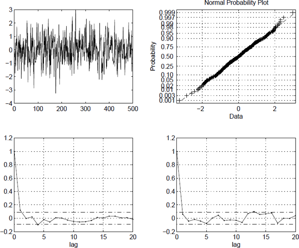
Sample autocorrelation and QQ plot for the generalized Gaussian residuals computed for the Cox-Ingersoll-Ross process.
The benchmark for stocks is the geometric Brownian motion, dS(t) = μS(t)dt + σS(t)dW(t). Let Δk = tk − tk−1 be the sampling interval and let ΔWi=Wtk−Wtk−1,˜μ=(μ−σ2/2). The solution to the stochastic differential equation is given by Stk=Stk−1e˜μΔk+σΔWk. We obtain Uk by applying the distribution function. The conditional distribution of Stk is given by
ℙ(Stk−1e˜μΔk+σΔWk≤sk|Stk−1)=Φ(log(sk/Stk−1)−˜μΔkσ√Δk).
By applying the inverse of the distribution function of the standard Gaussian random variable, we find that
Yk=Φ−1(Uk)=log(sk/Stk−1)−˜μΔkσ√Δk.
The generalized Gaussian residuals are consistent with the ordinary standardized residuals (for linear diffusions) but the technique is also able to handle non-linear models. We have calculated the generalized Gaussian residuals for the S & P 500 using weekly data from 1983–2002. The residuals are presented in Figure 13.5. It can be seen that the residuals are non-Gaussian and heteroscedastic, reaffirming the well-known fact that the S & P 500 is not generated by a geometric Brownian motion.

Generalized Gaussian residuals (left) and QQ plot (right) for continuously compounded returns on the S & P 500.
13.8 Problems
Problem 13.1
Consider the stochastic variable X ∈ N(μ, σ2).
- 1. Specify two moment conditions that can be used for estimating the parameters μ and σ2.
- 2. Specify an additional moment condition.
- 3. Simulate 100 observations of X. Estimate the parameters and their covariances based on these observations using the two moment conditions. Estimate the parameters and their covariances based on these observations using the three moment conditions. Comment on the results.
Problem 13.2
Consider the GARCH model (5.67) for p = 1 and q = 1, i.e., the GARCH(1,1) model.
- 1. Write down suitable moment conditions for estimating the parameters. Illustrate the choice of moment conditions!
Hint: Use (5.69).
Problem 13.3
Consider the CKLS model
dX(t)=κ(θ−X(t))dt+σX(t)γdW(t).
- 1. Calculate the simple estimation functions obtained from choosing h(x) = x2, x3, x4.
- 2. Do an Euler approximation of the CKLS model with timestep Δ. Use this to derive suitable moment conditions for a GMM estimation of the parameters.
1Similar results exist in the theory on discrete time series analysis.