Chapter 12
Discrete time approximations
In this chapter we introduce some basic issues concerning discrete time approximations of stochastic differential equations, which are used in a later chapter to estimate the parameters in SDEs using the Generalized Method of Moments (GMM). Furthermore the methods are used to simulate discrete observations from a continuous time system, which, for example, can be used to determine the price of a financial derivative in cases where no closed form solution of the pricing formula exist.
12.1 Stochastic Taylor expansion
The stochastic Taylor expansion is a stochastic counterpart of the Taylor expansion in a deterministic framework, and it is essential for the discrete time approximation of stochastic differential equations to be described later in this chapter. The stochastic Taylor expansion is based on an iterated application of the Itō formula. Due to the high complexity of the multi dimensional case we shall only consider one-dimensional stochastic differential equations (Kloeden and Platen [1995]).
Consider the integral form
X(t)=X(t0)+∫tt0μ(X(s))ds+∫tt0σ(X(x))dW(s)(12.1)
for t ∈ [t0, T], where it is assumed that the functions μ and σ are “sufficiently” smooth in the neighbourhood of X(t0). If we apply the Itō formula to the functions μ and σ, and assume that the functions are time homogeneous, we obtain the following
X(t)=Xt0+μ(X(t0))∫tt0ds+σ(X(t0))∫tt0dW(s)+R(12.2)R=∫tt0∫st0ℒ0μ(X(z))dzds+∫tt0∫st0ℒ1μ(X(z))dW(z)ds+∫tt0∫st0ℒ0σ(X(z))dzdW(s)+∫tt0∫st0ℒ1σ(X(z))dW(z)dW(s)(12.3)
where the operators ℒ0 and ℒ1 are defined as
ℒ0=μ∂∂X+12σ2∂2∂X2,(12.4)ℒ1=σ∂∂X.(12.5)
This is the most simple Taylor expansion, where Itō's formula is only used once. The deterministic integral in the Taylor expansion (12.2) is equal to the length of the discretization interval t − t0, and the stochastic integral is Gaussian with distribution N(0, t − t0).
By continuously expanding the integrands of the multiple integrals in the remainder R, multiple integrals with constant integrands will appear. For example if we use the Itō formula on the integrand ℒ1σ(X(z)) in (12.2) we get the following
x(t)=X(t0)+μ(X(t0))∫tt0ds+σ(X(t0))∫tt0dW(s)+ℒ1σ(X(t0))∫tt0∫st0dW(z)dW(s)+ˉR(12.6)
where the remainder ˉR is a sum of multiple integrals with non-constant integrands.
In Section 12.3 the Itō-Taylor expansion is used to obtain discrete time approximations with different degrees of accuracy. In the same manner, we can obtain more accurate Taylor approximations by including more multiple stochastic integrals in the Taylor expansion, because these integrals contain additional information about the sample path of the stochastic process.
12.2 Convergence
In order to get a measure of the amount of error introduced in the discrete time approximation, two definitions of convergence are stated in the following. The distinction between the two definitions refers to whether the continuoustime discretized stochastic process approximates the sample paths of (12.1) pathwise for all t, or if it just approximates the moments or some probabilistic properties of (12.1).
To measure the magnitude of the approximation error introduced by the pathwise approximation {Yδ (t)}, with maximum step size δ, of an Itō process {X(t)}, consider the absolute error criterion
ε=E[|X(T)−Yδ(T)|](12.7)
where the error is expressed as the expectation of the absolute value of the difference between the Itō process and the approximation at a finite terminal time T.
Definition 12.1 (Strong convergence).
A general time discrete approximation Yδ (t) with maximum step size δ converges strongly to X at time T if
limδ→0E[|X(T)−Yδ(T)|]=0,(12.8)
and if there exists a positive constant C, which does not depend on δ, and a finite δ0 > 0 such that
ε(δ)=E[|X(T)−Yδ(T)|]≤Cδα(12.9)
for each δ ∈ (0,δ0), then Yδ is said to converge strongly of order α > 0.
In many practical situations we do not need such a strong convergence as the pathwise approximation considered above. For instance, we may only be interested in the computation of moments, probabilities or other functionals of the Itō process. Since the requirements for such a simulation are not as demanding as for the pathwise approximations, it is natural and convenient to classify these approximations separately. For that purpose we define the concept of weak convergence.
Definition 12.2 (Weak convergence).
A general time discrete approximation Yδ with maximum step size δ converges weakly to X, at time T as δ ↓ 0, with respect to a class C of polynomials g: ℝd → ℝ if we have
limδ→0|E[g(X(T))]−E[g(Yδ(T))]|=0,(12.10)
and if there exists a positive constant D, which does not depend on δ, and a finite δ0 > 0 such that
ε(δ)=|E[g(X(T))]−E[g(Yδ(T))]|≤Dδβ(12.11)
for each δ ∈ (0, δ0), then Yδ is said to converge weakly of order β > 0.
In Kloeden and Platen [1995] it is shown that the strong and weak convergence criteria lead to the development of different discretization schemes. As we shall see in the following a given dicretization scheme usually has different orders of convergence with respect to the two criteria.
12.3 Discretization schemes
12.3.1 Strong Taylor approximations
12.3.1.1 Explicit Euler scheme
The simplest strong Taylor approximation is the Euler scheme, also called the Euler-Maryama scheme. It utilizes only the first two terms in the simple Taylor expansion (12.2), and it attains the order of strong convergence γ = 0.5. In the one-dimensional case the Euler scheme has the form
Yn+1=Yn+μ(Yn)Δ+σ(Yn)ΔW(12.12)
where
Δ=τn+1−τn(12.13)
is the length of the time discretization interval, and
ΔW=Wτn+1−Wτn(12.14)
is the N(0, Δ;) increment of the Wiener process W.
12.3.1.2 Milstein scheme
If we add one additional term to the Euler scheme, we obtain a scheme proposed by Milstein [1974], which is of order 1.0 strong convergence.
Yn+1=Yn+μ(Yn)Δ+σ(Yn)ΔW+12σ(Yn)σ′(Yn)[(ΔW)2−Δ](12.15)
where the prime denotes the derivative with respect to the state variable. It is readily seen that the Euler scheme and the Milstein scheme coincide if the diffusion term a is independent of the state variable, because then the last term in (12.15) drops out. Due to the fact that the multiple integral can be expressed as
∫tt0∫st0dW(z)dW(s)=12[ΔW]2−Δ](12.16)
the Milstein scheme appears to correspond with the stochastic Taylor expansion (12.6) — refer to Kloeden and Platen [1995] for details.
12.3.1.3 The order 1.5 strong Taylor scheme
The order 1.5 strong Taylor scheme is given by
Yn+1=Yn+μΔ+σΔW+12σσ′[(ΔW)2−Δ]+μ′σΔZ+12(μμ′+12σ2μ″)Δ2+(μσ′+12σ2σ″)[ΔWΔ−ΔZ]+12σ(σσ″+(σ′)2)[13(ΔW)2−Δ]ΔW(12.17)
where μ and σ are evaluated at Yn and ΔZ is a random variable representing the double stochastic integral
ΔZ=∫τn+1τn∫sτndW(s)ds.(12.18)
In Kloeden and Platen [1995] it is shown that ΔZ is normally distributed with zero mean and variance equal to 13Δ3. The covariance between ΔW and ΔZ is 12Δ2
12.3.2 Weak Taylor approximations
As with the strong approximations, the desired order of convergence determines where the Taylor expansion must be truncated. However, the weak convergence criterion only concerns probabilistic aspects of the sample path and not the sample path itself. Therefore, for a certain degree of convergence, the required number of terms of the expansion is less for the case of weak convergence than for the case of strong convergence if a certain degree of convergence is desired.
For example it can be shown that the Euler approximation attains the order of weak convergence β = 1.0, whereas it only attains the order α = 0.5 of strong convergence.
12.3.2.1 The order 2.0 weak Taylor scheme
The order 2.0 weak Taylor scheme is given by
Yn+1=Yn+μΔ+σΔW+12σσ′[(ΔW)2−Δ]+μ′σΔZ+12(μμ′+12σ2μ″)Δ2+(μσ′+12σ2σ″)[ΔWΔ−ΔZ].(12.19)
Compared with the order 1.5 strong Taylor scheme the order 2.0 weak Taylor scheme is simpler, even though the degree of convergence is higher.
12.3.3 Exponential approximation
Some attention has recently been given to so-called exponential schemes (Mora [2005]) as these are generally better for stiff systems. The methodology does only apply to models where the diffusion is independent of the state, reducing the applicability somewhat.
The idea is to approximate the diffusion by an Ornstein-Uhlenbeck process, rather than an arithmetic Brownian motion (cf. the explicit Euler scheme). This idea is far from new, as it was used in Madsen and Melgaard [1991], Kristensen and Madsen [2003]. The advantage of approximating using an Ornstein-Uhlenbeck process is increased stability and, for some schemes, increased rate of convergence. Here, we present the Euler-exponential scheme
Yn+1=eJ(μ)δ(Yn+(μ−J(μ))Yn)Δ+σΔW)(12.20)
where J(μ) is the Jacobian of μ. This is a first-order scheme, but a similar, second order version can be found in Mora [2005].
12.4 Multilevel Monte Carlo
Consider the standard problem of approximating an expectation, E [Φ(S(T))], with some numerical scheme, say the Euler-Maruyama scheme, {Sδt}tε[0,T], with δ = T/M. The error between the numerical approximation and the exact value is then given by
ε=1NN∑n=1Φ(Sδ))−E[Φ(S(T))].(12.21)
This error can be decomposed into
ε=(1NN∑n=1Φ(Sδ(T))−1NN∑n=1Φ(S(T)))︸Discretization bias+(1NN∑n=1Φ(S(T))−E[Φ(S(T))])︸Variance(12.22)
where the bias from the first term is ? (δ) and the variance from the second term is ?(1/N), leading to a mean squared error (MSE) of
MSE=c1δ2+c2N.(12.23)
Balancing these terms means that δ 2 ∝ 1/N. If the MSE equals ε2, the δ2 = ?(ε2) and 1/N = ?(ε2) which means that the complexity needed for a root mean squared error of size ε is
Complexity=MεNε=?(ε−1)?(ε−2)=?(ε−3).(12.24)
It turns out that this complexity can be reduced substantially to ?(ε−2(log(ε))2) by organizing the computations in a clever way (Giles [2008]), called MultiLevel Monte Carlo (MLMC).
Consider a simple approximation computed at the crudest possible scale, δ0 = T, computed using N0 samples. That approximation, called P0, will be severely biased but the complexity is low as only a single step is taken. The idea behind multilevel Monte Carlo is to compute a series of corrections with δl = M−1T (M being an integer) to this crude level. Denote the Monte Carlo approximation at level l using Nl samples by Pl. It then follows that the expected value of the sequence of approximations is
E[P0+L∑l=1(Pl−Pl−1)]=E[PL] (12.25)
which is the accuracy of the finest level of approximations. The question is if the sequence of approximations can be computed in a less expensive way. This can in fact be done, provided that ideas related to so-called control variates are used.
The correction term, Yl = Pl − Pl1, is computed from two different levels of discretization using the same Brownian path, as this will introduce a strong coupling between these approximations. The paths should be independent of the other levels of approximation. Straightforward calculations (Giles [2008] for details), show that the variance of the sequence of corrections ΣLl=1Yl is given by
Var[Yl]=L∑l=1N−1lVl (12.26)
where Vl is the variance computed for a single Brownian path while the computational cost is given by
Cost=L∑l=1Nlδ−1l (12.27)
It can be shown that the variance is minimized for a fixed computational cost when Nl∝√VlSl, and that Vl = ?(Sl).
The number of samples Nl needed to obtain an overall variance of ε2 is Nl = ?(Lδlε−2) while the corresponding bias, provided that an Euler-Maruyama scheme is used, is ?(δL). Hence, we can compute the number of levels needed as
?(M−LT)=ε(12.28)
leading to L = log(ε−1))/log(M) + ?(1). The total computational cost for achieving a MSE of at most 2ε2 would then be
Cost=L∑l=1Nlδ−1l=L∑l=1?(Lδlε−2)δ−1l=?(ε−2L2)=?(ε−2(log(ε))2).(12.29)
This is a remarkable result as the cost for a perfect algorithm without bias would be ?(ε−2). Variations of the multilevel Monte Carlo method have been applied to, e.g., American options (Belomestny et al. [2013]). For simulation of exit times, see Higham et al. [2013].
12.5 Simulation of SDEs
Since explicit solutions of stochastic differential equations do only exist in a limited number of cases, numerical solution methods must be used. Different numerical approaches have been proposed, such as Markov chain approximations where both the state and the time variables are discretized. However for simulation purposes we shall use discrete time approximations because they have been presented in this chapter. By choosing a sufficiently small length of the subinterval Δ, the discretization schemes above can be used to generate discrete observations of a continuous-time system.
To illustrate some aspects of the simulation of a time discrete approximation of an Itō process we shall examine a simple example.
Example 12.1. Consider the geometric Brownian motion
dX(t)=μX(t)dt+σX(t)dW(t),X(0)=x0>0.(12.30)
We know from Example 8.10 that the solution of (12.30) is given by
X(t)=x0exp((μ−12σ2)t+σW(t)).(12.31)
The knowledge of the explicit solution gives us the possibility of comparing the discretization schemes with the exact solution and to calculate the error. To simulate a trajectory of the Euler approximation of the geometric Brownian motion we simply start from the initial value Y(0) = X(0) and proceed recursively to generate the next value from
Yn+1=Yn+μYnΔ+σYnΔWn(12.32)
where ΔWn is the N(0, Δ) increment of the Wiener process in the interval with length Δ = τn − τn − 1, which we assume constant. The Milstein approximation of the Geometric Brownian Motion is given by
Yn+1=Yn+μYnΔ+σYnΔWn+12σ2Yn((ΔWn)2−Δ).(12.33)
For comparison, we can use (12.31) to determine the corresponding values of the exact solution for the same sample path of the Wiener process, obtaining
Xτn=x0exp((μ−12σ2)τn+σn∑i=1ΔWi−1).(12.34)
In Figure 12.1 the exact process as well as the Euler and Milstein approximation are plotted for different values of the interval length Δ. It is readily seen that the approximations become better as the number ofsubintervals increases. Furthermore it is seen, as expected, that the Milstein scheme provides a better approximation than the Euler scheme.

Euler and Milstein approximation and the exact solution to (12.31) with initial value X(0) = 1, drift parameter μ = 1 and diffusion parameter σ = 1 for Δ=15 (upper plot) and Δ=115 (lower plot).
Example 12.2
Valuation of European call options in the Black & Scholes universe was covered in Chapter 9. Here, we have valuation options using Monte Carlo. The model we consider is given by
dS(t)=rS(t)dt+σS(t)dW(t)(12.35)
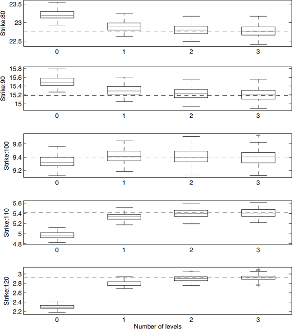
with S0 = 100, r = 0.4 and σ = 0.3. The time to maturity was T = 0.5, while the strike was varied between 80 and 120 in steps of 10. We consider four different cases:
- Exact value, computed using Equation (9.45) and (9.46).
- Crude Monte Carlo, using Euler-Maruyama without subsampling.
- Monte Carlo simulation using exact simulation, i.e., using the solution to the geometric Brownian motion.
- Multilevel Monte Carlo, using M = 4.
All Monte Carlo algorithms used the same number of random samples (in all N = 21 760 samples) in order to make the results comparable.
The resulting call prices are presented in Figure 12.2. It can be seen that the exact Monte Carlo is unbiased, the multilevel Monte Carlo is virtually unbiased, while the crude Monte Carlo is clearly biased (but the sign of the bias depends on the contract). The variance is roughly the same for all methods.
The convergence of the multilevel Monte Carlo for different levels of refinement is shown in Figure 12.3. It can be seen that just a few correction terms are usually enough to obtain nearly unbiased results.
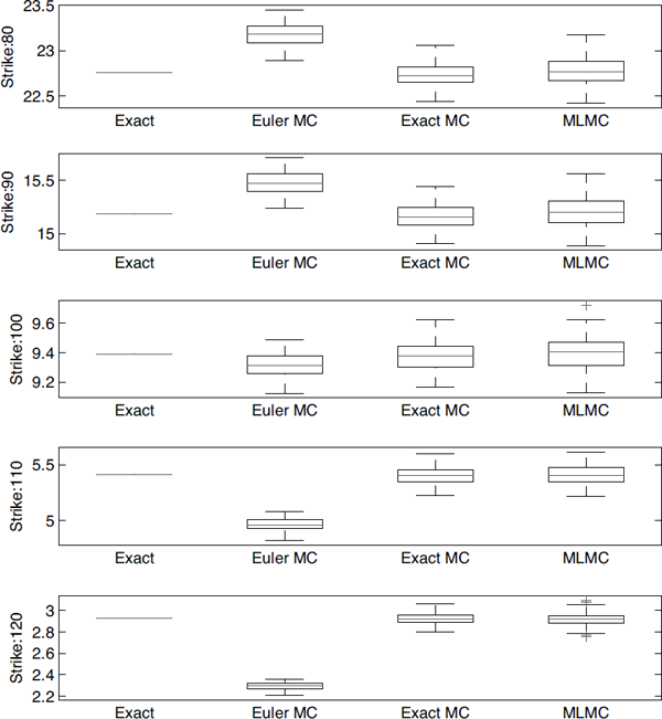
Prices for a European call option computed using the exact formula, an Euler-Maruyama scheme without subsampling, exact Monte Carlo and multilevel Monte Carlo.