
Chapter 10
k-Nearest Neighbor Algorithm
10.1 Classification Task
Perhaps the most common data mining task is that of classification. Examples of classification tasks may be found in nearly every field of endeavor:
- Banking: Determining whether a mortgage application is a good or bad credit risk, or whether a particular credit card transaction is fraudulent.
- Education: Placing a new student into a particular track with regard to special needs.
- Medicine: Diagnosing whether a particular disease is present.
- Law: Determining whether a will was written by the actual person deceased or fraudulently by someone else.
- Homeland security: Identifying whether or not certain financial or personal behavior indicates a possible terrorist threat.
In classification, there is a target categorical variable, (e.g., income bracket), which is partitioned into predetermined classes or categories, such as high income, middle income, and low income. The data mining model examines a large set of records, each record containing information on the target variable as well as a set of input or predictor variables. For example, consider the excerpt from a data set shown in Table 10.1. Suppose that the researcher would like to be able to classify the income bracket of persons not currently in the database, based on the other characteristics associated with that person, such as age, gender, and occupation. This task is a classification task, very nicely suited to data mining methods and techniques.
Table 10.1 Excerpt from data set for classifying income
| Subject | Age | Gender | Occupation | Income Bracket |
| 001 | 47 | F | Software engineer | High |
| 002 | 28 | M | Marketing consultant | Middle |
| 003 | 35 | M | Unemployed | Low |
The algorithm would proceed roughly as follows. First, examine the data set containing both the predictor variables and the (already classified) target variable, income bracket. In this way, the algorithm (software) “learns about” which combinations of variables are associated with which income brackets. For example, older females may be associated with the high-income bracket. This data set is called the training set. Then the algorithm would look at new records for which no information about income bracket is available. Based on the classifications in the training set, the algorithm would assign classifications to the new records. For example, a 63-year-old female professor might be classified in the high-income bracket.
10.2 k-Nearest Neighbor Algorithm
The first algorithm we shall investigate is the k-nearest neighbor algorithm, which is most often used for classification, although it can also be used for estimation and prediction. k-Nearest neighbor is an example of instance-based learning, in which the training data set is stored, so that a classification for a new unclassified record may be found simply by comparing it to the most similar records in the training set. Let us consider an example.
Recall the example from Chapter 1 where we were interested in classifying the type of drug a patient should be prescribed, based on certain patient characteristics, such as the age of the patient and the patient's sodium/potassium ratio. For a sample of 200 patients, Figure 10.1 presents a scatter plot of the patients' sodium/potassium (Na/K) ratio against the patients' ages. The particular drug prescribed is symbolized by the shade of the points. Light gray points indicate drug Y; medium gray points indicate drug A or X; dark gray points indicate drug B or C.
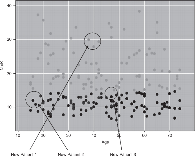
Figure 10.1 Scatter plot of sodium/potassium ratio against age, with drug overlay.
Now suppose that we have a new patient record, without a drug classification, and would like to classify which drug should be prescribed for the patient based on which drug was prescribed for other patients with similar attributes. Identified as “new patient 1,” this patient is 40 years old and has a Na/K ratio of 29, placing her at the center of the circle indicated for new patient 1 in Figure 10.1. Which drug classification should be made for new patient 1? Since her patient profile places her deep into a section of the scatter plot where all patients are prescribed drug Y, we would thereby classify new patient 1 as drug Y. All of the points nearest to this point, that is, all of the patients with a similar profile (with respect to age and Na/K ratio) have been prescribed the same drug, making this an easy classification.
Next, we move to new patient 2, who is 17 years old with a Na/K ratio of 12.5. Figure 10.2 provides a close-up view of the training data points in the local neighborhood of and centered at new patient 2. Suppose we let k = 1 for our k-nearest neighbor algorithm, so that new patient 2 would be classified according to whichever single (one) observation it was closest to. In this case, new patient 2 would be classified for drugs B and C (dark gray), since that is the classification of the point closest to the point on the scatter plot for new patient 2.
Figure 10.2 Close-up of three nearest neighbors to new patient 2.
However, suppose that we now let k = 2 for our k-nearest neighbor algorithm, so that new patient 2 would be classified according to the classification of the k = 2 points closest to it. One of these points is dark gray, and one is medium gray, so that our classifier would be faced with a decision between classifying new patient 2 for drugs B and C (dark gray) or drugs A and X (medium gray). How would the classifier decide between these two classifications? Voting would not help, since there is one vote for each of the two classifications.
Voting would help, however, if we let k = 3 for the algorithm, so that new patient 2 would be classified based on the three points closest to it. Since two of the three closest points are medium gray, a classification based on voting would therefore choose drugs A and X (medium gray) as the classification for new patient 2. Note that the classification assigned for new patient 2 differed based on which value we chose for k.
Finally, consider new patient 3, who is 47 years old and has a Na/K ratio of 13.5. Figure 10.3 presents a close-up of the three nearest neighbors to new patient 3. For k = 1, the k-nearest neighbor algorithm would choose the dark gray (drugs B and C) classification for new patient 3, based on a distance measure. For k = 2, however, voting would not help. But voting would not help for k = 3 in this case either, since the three nearest neighbors to new patient 3 are of three different classifications.

Figure 10.3 Close-up of three nearest neighbors to new patient 3.
This example has shown us some of the issues involved in building a classifier using the k-nearest neighbor algorithm. These issues include
- How many neighbors should we consider? That is, what is k?
- How do we measure distance?
- How do we combine the information from more than one observation?
Later we consider other questions, such as
- Should all points be weighted equally, or should some points have more influence than others?
10.3 Distance Function
We have seen above how, for a new record, the k-nearest neighbor algorithm assigns the classification of the most similar record or records. But just how do we define similar? For example, suppose that we have a new patient who is a 50-year-old male. Which patient is more similar, a 20-year-old male or a 50-year-old female?
Data analysts define distance metrics to measure similarity. A distance metric or distance function is a real-valued function d, such that for any coordinates x, y, and z:
- d(x,y) ≥ 0, and d(x,y) = 0 if and only if x = y;
- d(x,y) = d(y,x);
- d(x,z) ≤ d(x,y) + d(y,z).
Property 1 assures us that distance is always nonnegative, and the only way for distance to be zero is for the coordinates (e.g., in the scatter plot) to be the same. Property 2 indicates commutativity, so that, for example, the distance from New York to Los Angeles is the same as the distance from Los Angeles to New York. Finally, property 3 is the triangle inequality, which states that introducing a third point can never shorten the distance between two other points.
The most common distance function is Euclidean distance, which represents the usual manner in which humans think of distance in the real world:
where x = x1, x2,…, xm and y = y1, y2,…, ym represent the m attribute values of two records. For example, suppose that patient A is x1 = 20 years old and has a Na/K ratio of x2 = 12, while patient B is y1 = 30 years old and has a Na/K ratio of y2 = 8. Then the Euclidean distance between these points, as shown in Figure 10.4, is
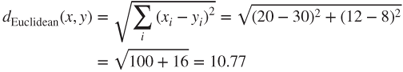

Figure 10.4 Euclidean distance.
When measuring distance, however, certain attributes that have large values, such as income, can overwhelm the influence of other attributes that are measured on a smaller scale, such as years of service. To avoid this, the data analyst should make sure to normalize the attribute values.
For continuous variables, the min–max normalization or Z-score standardization, discussed in Chapter 2, may be used:
Min–max normalization:
Z-score standardization:
For categorical variables, the Euclidean distance metric is not appropriate. Instead, we may define a function, “different from,” used to compare the ith attribute values of a pair of records, as follows:

where xi and yi are categorical values. We may then substitute different (xi, yi) for the ith term in the Euclidean distance metric above.
For example, let us find an answer to our earlier question: Which patient is more similar to a 50-year-old male: a 20-year-old male or a 50-year-old female? Suppose that for the age variable, the range is 50, the minimum is 10, the mean is 45, and the standard deviation is 15. Let patient A be our 50-year-old male, patient B the 20-year-old male, and patient C the 50-year-old female. The original variable values, along with the min–max normalization (ageMMN) and Z-score standardization (ageZscore), are listed in Table 10.2.
Table 10.2 Variable values for age and gender
| Patient | Age | AgeMMN | AgeZscore | Gender |
| A | 50 | Male | ||
| B | 20 | Male | ||
| C | 50 | Female |
We have one continuous variable (age, x1) and one categorical variable (gender, x2). When comparing patients A and B, we have different (x2, y2) = 0, with different (x2, y2) = 1 for the other combinations of patients. First, let us see what happens when we forget to normalize the age variable. Then, the distance between patients A and B is ![]() , and the distance between patients A and C is
, and the distance between patients A and C is ![]() . We would thus conclude that the 20-year-old male is 30 times more “distant” from the 50-year-old male than the 50-year-old female is. In other words, the 50-year-old female is 30 times more “similar” to the 50-year-old male than the 20-year-old male is. Does this seem justified to you? Well, in certain circumstances, it may be justified, as in certain age-related illnesses. But, in general, one may judge that the two men are just as similar as are the two 50-year-olds. The problem is that the age variable is measured on a larger scale than the different(x2, y2) variable. Therefore, we proceed to account for this discrepancy by normalizing and standardizing the age values, as shown in Table 10.2.
. We would thus conclude that the 20-year-old male is 30 times more “distant” from the 50-year-old male than the 50-year-old female is. In other words, the 50-year-old female is 30 times more “similar” to the 50-year-old male than the 20-year-old male is. Does this seem justified to you? Well, in certain circumstances, it may be justified, as in certain age-related illnesses. But, in general, one may judge that the two men are just as similar as are the two 50-year-olds. The problem is that the age variable is measured on a larger scale than the different(x2, y2) variable. Therefore, we proceed to account for this discrepancy by normalizing and standardizing the age values, as shown in Table 10.2.
Next, we use the min–max normalization values to find which patient is more similar to patient A. We have ![]() and
and ![]() , which means that patient B is now considered to be more similar to patient A.
, which means that patient B is now considered to be more similar to patient A.
Finally, we use the Z-score standardization values to determine which patient is more similar to patient A. We have ![]() and
and ![]() , which means that patient C is closer. Using the Z-score standardization rather than the min–max standardization has reversed our conclusion about which patient is considered to be more similar to patient A. This underscores the importance of understanding which type of normalization one is using. The min–max normalization will almost always lie between zero and 1 just like the “identical” function. The Z-score standardization, however, usually takes values −3 < z < 3, representing a wider scale than that of the min–max normalization. Therefore, perhaps, when mixing categorical and continuous variables, the min–max normalization may be preferred.
, which means that patient C is closer. Using the Z-score standardization rather than the min–max standardization has reversed our conclusion about which patient is considered to be more similar to patient A. This underscores the importance of understanding which type of normalization one is using. The min–max normalization will almost always lie between zero and 1 just like the “identical” function. The Z-score standardization, however, usually takes values −3 < z < 3, representing a wider scale than that of the min–max normalization. Therefore, perhaps, when mixing categorical and continuous variables, the min–max normalization may be preferred.
10.4 Combination Function
Now that we have a method of determining which records are most similar to the new, unclassified record, we need to establish how these similar records will combine to provide a classification decision for the new record. That is, we need a combination function. The most basic combination function is simple unweighted voting.
10.4.1 Simple Unweighted Voting
- Before running the algorithm, decide on the value of k, that is, how many records will have a voice in classifying the new record.
- Then, compare the new record to the k nearest neighbors, that is, to the k records that are of minimum distance from the new record in terms of the Euclidean distance or whichever metric the user prefers.
- Once the k records have been chosen, then for simple unweighted voting, their distance from the new record no longer matters. It is simple one record, one vote.
We observed simple unweighted voting in the examples for Figures 10.2 and 10.3. In Figure 10.2, for k = 3, a classification based on simple voting would choose drugs A and X (medium gray) as the classification for new patient 2, as two of the three closest points are medium gray. The classification would then be made for drugs A and X, with confidence 66.67%, where the confidence level represents the count of records, with the winning classification divided by k.
However, in Figure 10.3, for k = 3, simple voting would fail to choose a clear winner as each of the three categories receives one vote. There would be a tie among the three classifications represented by the records in Figure 10.3, and a tie may not be a preferred result.
10.4.2 Weighted Voting
One may feel that neighbors that are closer or more similar to the new record should be weighted more heavily than more distant neighbors. For example, in Figure 10.3, does it seem fair that the light gray record farther away gets the same vote as the dark gray vote that is closer to the new record? Perhaps not. Instead, the analyst may choose to apply weighted voting, where closer neighbors have a larger voice in the classification decision than do more distant neighbors. Weighted voting also makes it much less likely for ties to arise.
In weighted voting, the influence of a particular record is inversely proportional to the distance of the record from the new record to be classified. Let us look at an example. Consider Figure 10.2, where we are interested in finding the drug classification for a new record, using the k = 3 nearest neighbors. Earlier, when using simple unweighted voting, we saw that there were two votes for the medium gray classification, and one vote for the dark gray. However, the dark gray record is closer than the other two records. Will this greater proximity be enough for the influence of the dark gray record to overcome that of the more numerous medium gray records?
Assume that the records in question have the values for age and Na/K ratio given in Table 10.3, which also shows the min–max normalizations for these values. Then the distances of records A, B, and C from the new record are as follows:
The votes of these records are then weighted according to the inverse square of their distances.
Table 10.3 Age and Na/K ratios for records from Figure 5.4
| Record | Age | Na/K | AgeMMN | Na/KMMN |
| New | 17 | 12.5 | 0.05 | 0.25 |
| A (dark gray) | 16.8 | 12.4 | 0.0467 | 0.2471 |
| B (medium gray) | 17.2 | 10.5 | 0.0533 | 0.1912 |
| C (medium gray) | 19.5 | 13.5 | 0.0917 | 0.2794 |
One record (A) votes to classify the new record as dark gray (drugs B and C), so the weighted vote for this classification is
Two records (B and C) vote to classify the new record as medium gray (drugs A and X), so the weighted vote for this classification is
Therefore, by the convincing total of 51,818 to 672, the weighted voting procedure would choose dark gray (drugs B and C) as the classification for a new 17-year-old patient with a sodium/potassium ratio of 12.5. Note that this conclusion reverses the earlier classification for the unweighted k = 3 case, which chose the medium gray classification.
When the distance is zero, the inverse would be undefined. In this case, the algorithm should choose the majority classification of all records whose distance is zero from the new record.
Consider for a moment that once we begin weighting the records, there is no theoretical reason why we could not increase k arbitrarily so that all existing records are included in the weighting. However, this runs up against the practical consideration of very slow computation times for calculating the weights of all of the records every time a new record needs to be classified.
10.5 Quantifying Attribute Relevance: Stretching the Axes
Consider that not all attributes may be relevant to the classification. In decision trees (Chapter 11), for example, only those attributes that are helpful to the classification are considered. In the k-nearest neighbor algorithm, the distances are by default calculated on all the attributes. It is possible, therefore, for relevant records that are proximate to the new record in all the important variables, but are distant from the new record in unimportant ways, to have a moderately large distance from the new record, and therefore not be considered for the classification decision. Analysts may therefore consider restricting the algorithm to fields known to be important for classifying new records, or at least to blind the algorithm to known irrelevant fields.
Alternatively, rather than restricting fields a priori, the data analyst may prefer to indicate which fields are of more or less importance for classifying the target variable. This can be accomplished using a cross-validation approach or one based on domain expert knowledge. First, note that the problem of determining which fields are more or less important is equivalent to finding a coefficient zj by which to multiply the jth axis, with larger values of zj associated with more important variable axes. This process is therefore termed stretching the axes.
The cross-validation approach then selects a random subset of the data to be used as a training set and finds the set of values z1, z2,…, zm that minimize the classification error on the test data set. Repeating the process will lead to a more accurate set of values z1, z2,…, zm. Otherwise, domain experts may be called on to recommend a set of values for z1, z2,…, zm. In this way, the k-nearest neighbor algorithm may be made more precise.
For example, suppose that either through cross-validation or expert knowledge, the Na/K ratio was determined to be three times as important as age for drug classification. Then we would have zNa/K = 3 and zage = 1. For the example above, the new distances of records A, B, and C from the new record would be as follows:

In this case, the classification would not change with the stretched axis for Na/K, remaining dark gray. In real-world problems, however, axis stretching can lead to more accurate classifications, as it represents a method for quantifying the relevance of each variable in the classification decision.
10.6 Database Considerations
For instance-based learning methods such as the k-nearest neighbor algorithm, it is vitally important to have access to a rich database full of as many different combinations of attribute values as possible. It is especially important that rare classifications be represented sufficiently, so that the algorithm does not only predict common classifications. Therefore, the data set would need to be balanced, with a sufficiently large percentage of the less common classifications. One method to perform balancing is to reduce the proportion of records with more common classifications.
Maintaining this rich database for easy access may become problematic if there are restrictions on main memory space. Main memory may fill up, and access to auxiliary storage is slow. Therefore, if the database is to be used for k-nearest neighbor methods only, it may be helpful to retain only those data points that are near a classification “boundary.” For example, in Figure 10.1, all records with Na/K ratio value greater than, say, 19 could be omitted from the database without loss of classification accuracy, as all records in this region are classified as light gray. New records with Na/K ratio >19 would therefore be classified similarly.
10.7 k-Nearest Neighbor Algorithm for Estimation and Prediction
So far we have considered how to use the k-nearest neighbor algorithm for classification. However, it may be used for estimation and prediction as well as for continuous-valued target variables. One method for accomplishing this is called locally weighted averaging. Assume that we have the same data set as the example above, but this time rather than attempting to classify the drug prescription, we are trying to estimate the systolic blood pressure reading (BP, the target variable) of the patient, based on that patient's age and Na/K ratio (the predictor variables). Assume that BP has a range of 80 with a minimum of 90 in the patient records.
In this example, we are interested in estimating the systolic BP reading for a 17-year-old patient with a Na/K ratio of 12.5, the same new patient record for which we earlier performed drug classification. If we let k = 3, we have the same three nearest neighbors as earlier, shown here in Table 10.4. Assume that we are using the zNa/K = three-axis-stretching to reflect the greater importance of the Na/K ratio.
Table 10.4 k = 3 nearest neighbors of the new record
| Record | Age | Na/K | BP | AgeMMN | Na/KMMN | Distance |
| New | 17 | 12.5 | ? | 0.05 | 0.25 | — |
| A | 16.8 | 12.4 | 120 | 0.0467 | 0.2471 | 0.009305 |
| B | 17.2 | 10.5 | 122 | 0.0533 | 0.1912 | 0.17643 |
| C | 19.5 | 13.5 | 130 | 0.0917 | 0.2794 | 0.26737 |
Locally weighted averaging would then estimate BP as the weighted average of BP for the k = 3 nearest neighbors, using the same inverse square of the distances for the weights that we used earlier. That is, the estimated target value ![]() is calculated as
is calculated as
where ![]() for existing records x1, x2,…, xk. Thus, in this example, the estimated systolic BP reading for the new record would be
for existing records x1, x2,…, xk. Thus, in this example, the estimated systolic BP reading for the new record would be
As expected, the estimated BP value is quite close to the BP value in the present data set that is much closer (in the stretched attribute space) to the new record. In other words, as record A is closer to the new record, its BP value of 120 contributes greatly to the estimation of the BP reading for the new record.
10.8 Choosing k
How should one go about choosing the value of k? In fact, there may not be an obvious best solution. Consider choosing a small value for k. Then it is possible that the classification or estimation may be unduly affected by outliers or unusual observations (“noise”). With small k (e.g., k = 1), the algorithm will simply return the target value of the nearest observation, a process that may lead the algorithm toward overfitting, tending to memorize the training data set at the expense of generalizability.
However, choosing a value of k that is not too small will tend to smooth out any idiosyncratic behavior learned from the training set. However, if we take this too far and choose a value of k that is too large, locally interesting behavior will be overlooked. The data analyst needs to balance these considerations when choosing the value of k.
It is possible to allow the data itself to help resolve this problem, by following a cross-validation procedure similar to the earlier method for finding the optimal values z1, z2,…, zm for axis stretching. Here, we would try various values of k with different randomly selected training sets and choose the value of k that minimizes the classification or estimation error.
10.9 Application of k-Nearest Neighbor Algorithm Using IBM/SPSS Modeler
Table 10.5 contains a small data set of 10 records excerpted from the ClassifyRisk data set, with predictors' age, marital status, and income, and target variable risk. We seek the k-nearest neighbor for record 10, using k = 2. Modeler's results are shown in Figure 10.5. (Note that Modeler automatically normalizes the data.) Records 8 and 9 are the two nearest neighbors to Record 10, with the same marital status, and somewhat similar ages. As both Records 8 and 9 and classified as Good risk, the prediction for Record 10 would be Good risk as well.
Table 10.5 Find the k-nearest neighbor for Record #10
| Record | Age | Marital | Income | Risk |
| 1 | 22 | Single | $46,156.98 | Bad loss |
| 2 | 33 | Married | $24,188.10 | Bad loss |
| 3 | 28 | Other | $28,787.34 | Bad loss |
| 4 | 51 | Other | $23,886.72 | Bad loss |
| 5 | 25 | Single | $47,281.44 | Bad loss |
| 6 | 39 | Single | $33,994.90 | Good risk |
| 7 | 54 | Single | $28,716.50 | Good risk |
| 8 | 55 | Married | $49,186.75 | Good risk |
| 9 | 50 | Married | $46,726.50 | Good risk |
| 10 | 66 | Married | $36,120.34 | Good risk |
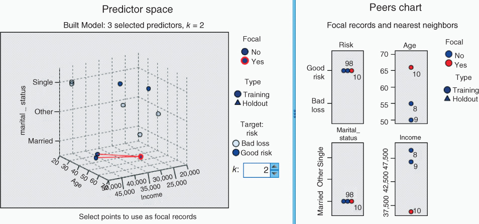
Figure 10.5 Modeler k-nearest neighbor results.
R References
- R Core Team (2012). R: A Language and Environment for Statistical Computing. R Foundation for Statistical Computing, Vienna, Austria. 3-900051-07-0, http://www.R-project.org/.
- Venables WN, Ripley BD. Modern Applied Statistics with S. 4th ed. New York: Springer; 2002. ISBN: 0-387-95457-0.
Exercises
1. Clearly describe what is meant by classification.
2. What is meant by the term instance-based learning?
3. Make up a set of three records, each with two numeric predictor variables and one categorical target variable, so that the classification would not change regardless of the value of k.
4. Refer to Exercise 3. Alter your data set so that the classification changes for different values of k.
5. Refer to Exercise 4. Find the Euclidean distance between each pair of points. Using these points, verify that Euclidean distance is a true distance metric.
6. Compare the advantages and drawbacks of unweighted versus weighted voting.
7. Why does the database need to be balanced?
8. The example in the text regarding using the k-nearest neighbor algorithm for estimation has the closest record, overwhelming the other records in influencing the estimation. Suggest two creative ways that we could use to dilute this strong influence of the closest record.
9. Discuss the advantages and drawbacks of using a small value versus a large value for k.
10. Why would one consider stretching the axes?
11. What is locally weighted averaging, and how does it help in estimation?
Hands-On Analysis
12. Using the data in table 10.5, find the k-nearest neighbor for Record #10, using k = 3.
13. Using the ClassifyRisk data set with predictors age, marital status, and income, and target variable risk, find the k-nearest neighbor for Record #1, using k = 2 and Euclidean distance.
14. Using the ClassifyRisk data set with predictors age, marital status, and income, and target variable risk, find the k-nearest neighbor for Record #1, using k = 2 and Minkowski (city-block) distance (Chapter 19).