
Chapter 1
An Introduction to Data Mining and Predictive Analytics
1.1 What is Data Mining? What Is Predictive Analytics?
Recently, the computer manufacturer Dell was interested in improving the productivity of its sales workforce. It therefore turned to data mining and predictive analytics to analyze its database of potential customers, in order to identify the most likely respondents. Researching the social network activity of potential leads, using LinkedIn and other sites, provided a richer amount of information about the potential customers, thereby allowing Dell to develop more personalized sales pitches to their clients. This is an example of mining customer data to help identify the type of marketing approach for a particular customer, based on customer's individual profile. What is the bottom line? The number of prospects that needed to be contacted was cut by 50%, leaving only the most promising prospects, leading to a near doubling of the productivity and efficiency of the sales workforce, with a similar increase in revenue for Dell.1
The Commonwealth of Massachusetts is wielding predictive analytics as a tool to cut down on the number of cases of Medicaid fraud in the state. When a Medicaid claim is made, the state now immediately passes it in real time to a predictive analytics model, in order to detect any anomalies. During its first 6 months of operation, the new system has “been able to recover $2 million in improper payments, and has avoided paying hundreds of thousands of dollars in fraudulent claims,” according to Joan Senatore, Director of the Massachusetts Medicaid Fraud Unit.2
The McKinsey Global Institute (MGI) reports3 that most American companies with more than 1000 employees had an average of at least 200 TB of stored data. MGI projects that the amount of data generated worldwide will increase by 40% annually, creating profitable opportunities for companies to leverage their data to reduce costs and increase their bottom line. For example, retailers harnessing this “big data” to best advantage could expect to realize an increase in their operating margin of more than 60%, according to the MGI report. And health-care providers and health maintenance organizations (HMOs) that properly leverage their data storehouses could achieve $300 in cost savings annually, through improved efficiency and quality.
Forbes magazine reports4 that the use of data mining and predictive analytics has helped to identify patients who have been of the greatest risk of developing congestive heart failure. IBM collected 3 years of data pertaining to 350,000 patients, and including measurements on over 200 factors, including things such as blood pressure, weight, and drugs prescribed. Using predictive analytics, IBM was able to identify the 8500 patients most at risk of dying of congestive heart failure within 1 year.
The MIT Technology Review reports5 that it was the Obama campaign's effective use of data mining that helped President Obama win the 2012 presidential election over Mitt Romney. They first identified likely Obama voters using a data mining model, and then made sure that these voters actually got to the polls. The campaign also used a separate data mining model to predict the polling outcomes county by county. In the important swing county of Hamilton County, Ohio, the model predicted that Obama would receive 56.4% of the vote; the Obama share of the actual vote was 56.6%, so that the prediction was off by only 0.02%. Such precise predictive power allowed the campaign staff to allocate scarce resources more efficiently.
So, what is data mining? What is predictive analytics?
While waiting in line at a large supermarket, have you ever just closed your eyes and listened? You might hear the beep, beep, beep of the supermarket scanners, reading the bar codes on the grocery items, ringing up on the register, and storing the data on company servers. Each beep indicates a new row in the database, a new “observation” in the information being collected about the shopping habits of your family, and the other families who are checking out.
Clearly, a lot of data is being collected. However, what is being learned from all this data? What knowledge are we gaining from all this information? Probably not as much as you might think, because there is a serious shortage of skilled data analysts.
1.2 Wanted: Data Miners
As early as 1984, in his book Megatrends,6 John Naisbitt observed that “We are drowning in information but starved for knowledge.” The problem today is not that there is not enough data and information streaming in. We are in fact inundated with data in most fields. Rather, the problem is that there are not enough trained human analysts available who are skilled at translating all of this data into knowledge, and thence up the taxonomy tree into wisdom.
The ongoing remarkable growth in the field of data mining and knowledge discovery has been fueled by a fortunate confluence of a variety of factors:
- The explosive growth in data collection, as exemplified by the supermarket scanners above.
- The storing of the data in data warehouses, so that the entire enterprise has access to a reliable, current database.
- The availability of increased access to data from web navigation and intranets.
- The competitive pressure to increase market share in a globalized economy.
- The development of “off-the-shelf” commercial data mining software suites.
- The tremendous growth in computing power and storage capacity.
Unfortunately, according to the McKinsey report,7
There will be a shortage of talent necessary for organizations to take advantage of big data. A significant constraint on realizing value from big data will be a shortage of talent, particularly of people with deep expertise in statistics and machine learning, and the managers and analysts who know how to operate companies by using insights from big data… We project that demand for deep analytical positions in a big data world could exceed the supply being produced on current trends by 140,000 to 190,000 positions. … In addition, we project a need for 1.5 million additional managers and analysts in the United States who can ask the right questions and consume the results of the analysis of big data effectively.
This book is an attempt to help alleviate this critical shortage of data analysts.
1.3 The Need For Human Direction of Data Mining
Automation is no substitute for human oversight. Humans need to be actively involved at every phase of the data mining process. Rather than asking where humans fit into data mining, we should instead inquire about how we may design data mining into the very human process of problem solving.
Further, the very power of the formidable data mining algorithms embedded in the black box software currently available makes their misuse proportionally more dangerous. Just as with any new information technology, data mining is easy to do badly. Researchers may apply inappropriate analysis to data sets that call for a completely different approach, for example, or models may be derived that are built on wholly specious assumptions. Therefore, an understanding of the statistical and mathematical model structures underlying the software is required.
1.4 The Cross-Industry Standard Process for Data Mining: CRISP-DM
There is a temptation in some companies, due to departmental inertia and compartmentalization, to approach data mining haphazardly, to reinvent the wheel and duplicate effort. A cross-industry standard was clearly required, that is industry-neutral, tool-neutral, and application-neutral. The Cross-Industry Standard Process for Data Mining (CRISP-DM8) was developed by analysts representing Daimler-Chrysler, SPSS, and NCR. CRISP provides a nonproprietary and freely available standard process for fitting data mining into the general problem-solving strategy of a business or research unit.
According to CRISP-DM, a given data mining project has a life cycle consisting of six phases, as illustrated in Figure 1.1. Note that the phase-sequence is adaptive. That is, the next phase in the sequence often depends on the outcomes associated with the previous phase. The most significant dependencies between phases are indicated by the arrows. For example, suppose we are in the modeling phase. Depending on the behavior and characteristics of the model, we may have to return to the data preparation phase for further refinement before moving forward to the model evaluation phase.

Figure 1.1 CRISP-DM is an iterative, adaptive process.
The iterative nature of CRISP is symbolized by the outer circle in Figure 1.1. Often, the solution to a particular business or research problem leads to further questions of interest, which may then be attacked using the same general process as before. Lessons learned from past projects should always be brought to bear as input into new projects. Here is an outline of each phase. (Issues encountered during the evaluation phase can conceivably send the analyst back to any of the previous phases for amelioration.)
1.4.1 CRISP-DM: The Six Phases
- Business/Research Understanding Phase
- First, clearly enunciate the project objectives and requirements in terms of the business or research unit as a whole.
- Then, translate these goals and restrictions into the formulation of a data mining problem definition.
- Finally, prepare a preliminary strategy for achieving these objectives.
- Data Understanding Phase
- First, collect the data.
- Then, use exploratory data analysis to familiarize yourself with the data, and discover initial insights.
- Evaluate the quality of the data.
- Finally, if desired, select interesting subsets that may contain actionable patterns.
- Data Preparation Phase
- This labor-intensive phase covers all aspects of preparing the final data set, which shall be used for subsequent phases, from the initial, raw, dirty data.
- Select the cases and variables you want to analyze, and that are appropriate for your analysis.
- Perform transformations on certain variables, if needed.
- Clean the raw data so that it is ready for the modeling tools.
- Modeling Phase
- Select and apply appropriate modeling techniques.
- Calibrate model settings to optimize results.
- Often, several different techniques may be applied for the same data mining problem.
- May require looping back to data preparation phase, in order to bring the form of the data into line with the specific requirements of a particular data mining technique.
- Evaluation Phase
- The modeling phase has delivered one or more models. These models must be evaluated for quality and effectiveness, before we deploy them for use in the field.
- Also, determine whether the model in fact achieves the objectives set for it in phase 1.
- Establish whether some important facet of the business or research problem has not been sufficiently accounted for.
- Finally, come to a decision regarding the use of the data mining results.
- Deployment Phase
- Model creation does not signify the completion of the project. Need to make use of created models.
- Example of a simple deployment: Generate a report.
- Example of a more complex deployment: Implement a parallel data mining process in another department.
- For businesses, the customer often carries out the deployment based on your model.
This book broadly follows CRISP-DM, with some modifications. For example, we prefer to clean the data (Chapter 2) before performing exploratory data analysis (Chapter 3).
1.5 Fallacies of Data Mining
Speaking before the US House of Representatives Subcommittee on Technology, Information Policy, Intergovernmental Relations, and Census, Jen Que Louie, President of Nautilus Systems, Inc., described four fallacies of data mining.9 Two of these fallacies parallel the warnings we have described above.
- Fallacy 1. There are data mining tools that we can turn loose on our data repositories, and find answers to our problems.
- Reality. There are no automatic data mining tools, which will mechanically solve your problems “while you wait.” Rather data mining is a process. CRISP-DM is one method for fitting the data mining process into the overall business or research plan of action.
- Fallacy 2. The data mining process is autonomous, requiring little or no human oversight.
- Reality. Data mining is not magic. Without skilled human supervision, blind use of data mining software will only provide you with the wrong answer to the wrong question applied to the wrong type of data. Further, the wrong analysis is worse than no analysis, because it leads to policy recommendations that will probably turn out to be expensive failures. Even after the model is deployed, the introduction of new data often requires an updating of the model. Continuous quality monitoring and other evaluative measures must be assessed, by human analysts.
- Fallacy 3. Data mining pays for itself quite quickly.
- Reality. The return rates vary, depending on the start-up costs, analysis personnel costs, data warehousing preparation costs, and so on.
- Fallacy 4. Data mining software packages are intuitive and easy to use.
- Reality. Again, ease of use varies. However, regardless of what some software vendor advertisements may claim, you cannot just purchase some data mining software, install it, sit back, and watch it solve all your problems. For example, the algorithms require specific data formats, which may require substantial preprocessing. Data analysts must combine subject matter knowledge with an analytical mind, and a familiarity with the overall business or research model.
To the above list, we add three further common fallacies:
- Fallacy 5. Data mining will identify the causes of our business or research problems.
- Reality. The knowledge discovery process will help you to uncover patterns of behavior. Again, it is up to the humans to identify the causes.
- Fallacy 6. Data mining will automatically clean up our messy database.
- Reality. Well, not automatically. As a preliminary phase in the data mining process, data preparation often deals with data that has not been examined or used in years. Therefore, organizations beginning a new data mining operation will often be confronted with the problem of data that has been lying around for years, is stale, and needs considerable updating.
- Fallacy 7. Data mining always provides positive results.
- Reality. There is no guarantee of positive results when mining data for actionable knowledge. Data mining is not a panacea for solving business problems. But, used properly, by people who understand the models involved, the data requirements, and the overall project objectives, data mining can indeed provide actionable and highly profitable results.
The above discussion may have been termed what data mining cannot or should not do. Next we turn to a discussion of what data mining can do.
1.6 What Tasks can Data Mining Accomplish
The following listing shows the most common data mining tasks.
Data Mining Tasks
- Description
- Estimation
- Prediction
- Classification
- Clustering
- Association.
1.6.1 Description
Sometimes researchers and analysts are simply trying to find ways to describe patterns and trends lying within the data. For example, a pollster may uncover evidence that those who have been laid off are less likely to support the present incumbent in the presidential election. Descriptions of patterns and trends often suggest possible explanations for such patterns and trends. For example, those who are laid off are now less well-off financially than before the incumbent was elected, and so would tend to prefer an alternative.
Data mining models should be as transparent as possible. That is, the results of the data mining model should describe clear patterns that are amenable to intuitive interpretation and explanation. Some data mining methods are more suited to transparent interpretation than others. For example, decision trees provide an intuitive and human-friendly explanation of their results. However, neural networks are comparatively opaque to nonspecialists, due to the nonlinearity and complexity of the model.
High-quality description can often be accomplished with exploratory data analysis, a graphical method of exploring the data in search of patterns and trends. We look at exploratory data analysis in Chapter 3.
1.6.2 Estimation
In estimation, we approximate the value of a numeric target variable using a set of numeric and/or categorical predictor variables. Models are built using “complete” records, which provide the value of the target variable, as well as the predictors. Then, for new observations, estimates of the value of the target variable are made, based on the values of the predictors.
For example, we might be interested in estimating the systolic blood pressure reading of a hospital patient, based on the patient's age, gender, body mass index, and blood sodium levels. The relationship between systolic blood pressure and the predictor variables in the training set would provide us with an estimation model. We can then apply that model to new cases.
Examples of estimation tasks in business and research include
- estimating the amount of money a randomly chosen family of four will spend for back-to-school shopping this fall;
- estimating the percentage decrease in rotary movement sustained by a National Football League (NFL) running back with a knee injury;
- estimating the number of points per game LeBron James will score when double-teamed in the play-offs;
- estimating the grade point average (GPA) of a graduate student, based on that student's undergraduate GPA.
Consider Figure 1.2, where we have a scatter plot of the graduate GPAs against the undergraduate GPAs for 1000 students. Simple linear regression allows us to find the line that best approximates the relationship between these two variables, according to the least-squares criterion. The regression line, indicated in blue in Figure 1.2, may then be used to estimate the graduate GPA of a student, given that student's undergraduate GPA.
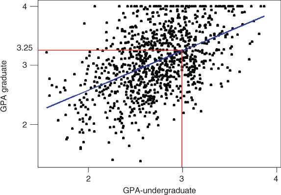
Figure 1.2 Regression estimates lie on the regression line.
Here, the equation of the regression line (as produced by the statistical package Minitab, which also produced the graph) is ![]() . This tells us that the estimated graduate GPA
. This tells us that the estimated graduate GPA ![]() equals 1.24 plus 0.67 times the student's undergrad GPA. For example, if your undergrad GPA is 3.0, then your estimated graduate GPA is
equals 1.24 plus 0.67 times the student's undergrad GPA. For example, if your undergrad GPA is 3.0, then your estimated graduate GPA is ![]() . Note that this point
. Note that this point ![]() lies precisely on the regression line, as do all of the linear regression predictions.
lies precisely on the regression line, as do all of the linear regression predictions.
The field of statistical analysis supplies several venerable and widely used estimation methods. These include point estimation and confidence interval estimations, simple linear regression and correlation, and multiple regression. We examine these methods and more in Chapters 5, 6, 8, and 9. Chapter 12 may also be used for estimation.
1.6.3 Prediction
Prediction is similar to classification and estimation, except that for prediction, the results lie in the future. Examples of prediction tasks in business and research include
- predicting the price of a stock 3 months into the future;
- predicting the percentage increase in traffic deaths next year if the speed limit is increased;
- predicting the winner of this fall's World Series, based on a comparison of the team statistics;
- predicting whether a particular molecule in drug discovery will lead to a profitable new drug for a pharmaceutical company.
Any of the methods and techniques used for classification and estimation may also be used, under appropriate circumstances, for prediction. These include the traditional statistical methods of point estimation and confidence interval estimations, simple linear regression and correlation, and multiple regression, investigated in Chapters 5, 6, 8, and 9, as well as data mining and knowledge discovery methods such as k-nearest neighbor methods (Chapter 10), decision trees (Chapter 11), and neural networks (Chapter 12).
1.6.4 Classification
Classification is similar to estimation, except that the target variable is categorical rather than numeric. In classification, there is a target categorical variable, such as income bracket, which, for example, could be partitioned into three classes or categories: high income, middle income, and low income. The data mining model examines a large set of records, each record containing information on the target variable as well as a set of input or predictor variables. For example, consider the excerpt from a data set in Table 1.1.
Table 1.1 Excerpt from dataset for classifying income
| Subject | Age | Gender | Occupation | Income Bracket |
| 001 | 47 | F | Software Engineer | High |
| 002 | 28 | M | Marketing Consultant | Middle |
| 003 | 35 | M | Unemployed | Low |
| … | … | … | … | … |
Suppose the researcher would like to be able to classify the income bracket of new individuals, not currently in the above database, based on the other characteristics associated with that individual, such as age, gender, and occupation. This task is a classification task, very nicely suited to data mining methods and techniques.
The algorithm would proceed roughly as follows. First, examine the data set containing both the predictor variables and the (already classified) target variable, income bracket. In this way, the algorithm (software) “learns about” which combinations of variables are associated with which income brackets. For example, older females may be associated with the high-income bracket. This data set is called the training set.
Then the algorithm would look at new records, for which no information about income bracket is available. On the basis of the classifications in the training set, the algorithm would assign classifications to the new records. For example, a 63-year-old female professor might be classified in the high-income bracket.
Examples of classification tasks in business and research include
- determining whether a particular credit card transaction is fraudulent;
- placing a new student into a particular track with regard to special needs;
- assessing whether a mortgage application is a good or bad credit risk;
- diagnosing whether a particular disease is present;
- determining whether a will was written by the actual deceased, or fraudulently by someone else;
- identifying whether or not certain financial or personal behavior indicates a possible terrorist threat.
For example, in the medical field, suppose we are interested in classifying the type of drug a patient should be prescribed, based on certain patient characteristics, such as the age of the patient, and the patient's sodium/potassium ratio. For a sample of 200 patients, Figure 1.3 presents a scatter plot of the patients' sodium/potassium ratio against the patients' age. The particular drug prescribed is symbolized by the shade of the points. Light gray points indicate drug Y; medium gray points indicate drugs A or X; dark gray points indicate drugs B or C. In this scatter plot, Na/K (sodium/potassium ratio) is plotted on the Y (vertical) axis and age is plotted on the X (horizontal) axis.

Figure 1.3 Which drug should be prescribed for which type of patient?
Suppose that we will base our prescription recommendation based on this data set.
- Which drug should be prescribed for a young patient with high sodium/ potassium ratio?
Young patients are on the left in the graph, and high sodium/potassium ratios are in the upper half, which indicates that previous young patients with high sodium/potassium ratios were prescribed drug Y (light gray points). The recommended prediction classification for such patients is drug Y.
- Which drug should be prescribed for older patients with low sodium/potassium ratios?
Patients in the lower right of the graph have been taking different prescriptions, indicated by either dark gray (drugs B or C) or medium gray (drugs A or X). Without more specific information, a definitive classification cannot be made here. For example, perhaps these drugs have varying interactions with beta-blockers, estrogens, or other medications, or are contraindicated for conditions such as asthma or heart disease.
Graphs and plots are helpful for understanding two- and three-dimensional relationships in data. But sometimes classifications need to be based on many different predictors, requiring a multidimensional plot. Therefore, we need to turn to more sophisticated models to perform our classification tasks. Common data mining methods used for classification are covered in Chapters 10–14.
1.6.5 Clustering
Clustering refers to the grouping of records, observations, or cases into classes of similar objects. A cluster is a collection of records that are similar to one another, and dissimilar to records in other clusters. Clustering differs from classification in that there is no target variable for clustering. The clustering task does not try to classify, estimate, or predict the value of a target variable. Instead, clustering algorithms seek to segment the whole data set into relatively homogeneous subgroups or clusters, where the similarity of the records within the cluster is maximized, and the similarity to records outside of this cluster is minimized.
Nielsen Claritas is in the clustering business. Among the services they provide is a demographic profile of each of the geographic areas in the country, as defined by zip code. One of the clustering mechanisms they use is the PRIZM segmentation system, which describes every American zip code area in terms of distinct lifestyle types. The 66 distinct clusters are shown in Table 1.2.
Table 1.2 The 66 clusters used by the PRIZM segmentation system
| 01 Upper Crust | 02 Blue Blood Estates | 03 Movers and Shakers |
| 04 Young Digerati | 05 Country Squires | 06 Winner's Circle |
| 07 Money and Brains | 08 Executive Suites | 09 Big Fish, Small Pond |
| 10 Second City Elite | 11 God's Country | 12 Brite Lites, Little City |
| 13 Upward Bound | 14 New Empty Nests | 15 Pools and Patios |
| 16 Bohemian Mix | 17 Beltway Boomers | 18 Kids and Cul-de-sacs |
| 19 Home Sweet Home | 20 Fast-Track Families | 21 Gray Power |
| 22 Young Influentials | 23 Greenbelt Sports | 24 Up-and-Comers |
| 25 Country Casuals | 26 The Cosmopolitans | 27 Middleburg Managers |
| 28 Traditional Times | 29 American Dreams | 30 Suburban Sprawl |
| 31 Urban Achievers | 32 New Homesteaders | 33 Big Sky Families |
| 34 White Picket Fences | 35 Boomtown Singles | 36 Blue-Chip Blues |
| 37 Mayberry-ville | 38 Simple Pleasures | 39 Domestic Duos |
| 40 Close-in Couples | 41 Sunset City Blues | 42 Red, White and Blues |
| 43 Heartlanders | 44 New Beginnings | 45 Blue Highways |
| 46 Old Glories | 47 City Startups | 48 Young and Rustic |
| 49 American Classics | 50 Kid Country, USA | 51 Shotguns and Pickups |
| 52 Suburban Pioneers | 53 Mobility Blues | 54 Multi-Culti Mosaic |
| 55Golden Ponds | 56 Crossroads Villagers | 57 Old Milltowns |
| 58 Back Country Folks | 59 Urban Elders | 60 Park Bench Seniors |
| 61 City Roots | 62 Hometown Retired | 63 Family Thrifts |
| 64 Bedrock America | 65 Big City Blues | 66 Low-Rise Living |
For illustration, the clusters for zip code 90210, Beverly Hills, California, are as follows:
- Cluster # 01: Upper Crust Estates
- Cluster # 03: Movers and Shakers
- Cluster # 04: Young Digerati
- Cluster # 07: Money and Brains
- Cluster # 16: Bohemian Mix.
The description for Cluster # 01: Upper Crust is “The nation's most exclusive address, Upper Crust is the wealthiest lifestyle in America, a haven for empty-nesting couples between the ages of 45 and 64. No segment has a higher concentration of residents earning over $100,000 a year and possessing a postgraduate degree. And none has a more opulent standard of living.”
Examples of clustering tasks in business and research include the following:
- Target marketing of a niche product for a small-cap business which does not have a large marketing budget.
- For accounting auditing purposes, to segmentize financial behavior into benign and suspicious categories.
- As a dimension-reduction tool when the data set has hundreds of attributes.
- For gene expression clustering, where very large quantities of genes may exhibit similar behavior.
Clustering is often performed as a preliminary step in a data mining process, with the resulting clusters being used as further inputs into a different technique downstream, such as neural networks. We discuss hierarchical and k-means clustering in Chapter 19, Kohonen networks in Chapter 20, and balanced iterative reducing and clustering using hierarchies (BIRCH) clustering in Chapter 21.
1.6.6 Association
The association task for data mining is the job of finding which attributes “go together.” Most prevalent in the business world, where it is known as affinity analysis or market basket analysis, the task of association seeks to uncover rules for quantifying the relationship between two or more attributes. Association rules are of the form “If antecedent then consequent,” together with a measure of the support and confidence associated with the rule. For example, a particular supermarket may find that, of the 1000 customers shopping on a Thursday night, 200 bought diapers, and of those 200 who bought diapers, 50 bought beer. Thus, the association rule would be “If buy diapers, then buy beer,” with a support of 200/1000 = 20% and a confidence of 50/200 = 25%.
Examples of association tasks in business and research include
- investigating the proportion of subscribers to your company's cell phone plan that respond positively to an offer of a service upgrade;
- examining the proportion of children whose parents read to them who are themselves good readers;
- predicting degradation in telecommunications networks;
- finding out which items in a supermarket are purchased together, and which items are never purchased together;
- determining the proportion of cases in which a new drug will exhibit dangerous side effects.
We discuss two algorithms for generating association rules, the a priori algorithm, and the generalized rule induction (GRI) algorithm, in Chapter 22.
R References
- Wickham H. ggplot2: Elegant Graphics for Data Analysis. New York: Springer; 2009.
- R Core Team. R: A Language and Environment for Statistical Computing. Vienna, Austria: R Foundation for Statistical Computing; 2012. ISBN: 3-900051-07-0, http://www.R-project.org/.
Exercises
1. For each of the following, identify the relevant data mining task(s):
- The Boston Celtics would like to approximate how many points their next opponent will score against them.
- A military intelligence officer is interested in learning about the respective proportions of Sunnis and Shias in a particular strategic region.
- A NORAD defense computer must decide immediately whether a blip on the radar is a flock of geese or an incoming nuclear missile.
- A political strategist is seeking the best groups to canvass for donations in a particular county.
- A Homeland Security official would like to determine whether a certain sequence of financial and residence moves implies a tendency to terrorist acts.
- A Wall Street analyst has been asked to find out the expected change in stock price for a set of companies with similar price/earnings ratios.
2. For each of the following meetings, explain which phase in the CRISP-DM process is represented:
- Managers want to know by next week whether deployment will take place. Therefore, analysts meet to discuss how useful and accurate their model is.
- The data mining project manager meets with the data warehousing manager to discuss how the data will be collected.
- The data mining consultant meets with the vice president for marketing, who says that he would like to move forward with customer relationship management.
- The data mining project manager meets with the production line supervisor, to discuss implementation of changes and improvements.
- The analysts meet to discuss whether the neural network or decision tree models should be applied.
3. Discuss the need for human direction of data mining. Describe the possible consequences of relying on completely automatic data analysis tools.
4. CRISP-DM is not the only standard process for data mining. Research an alternative methodology (Hint: Sample, Explore, Modify, Model and Assess (SEMMA), from the SAS Institute). Discuss the similarities and differences with CRISP-DM.