
Chapter 24
Segmentation Models
In Part 6: Enhancing Model Performance, we examine methods that enable us to enhance the performance of our models. Here in this chapter, we learn about Segmentation Models, where a useful clustering or subdivision of the data set is found, allowing us to develop cluster-specific models for each segment, and thereby enhancing the overall efficacy of the model. In Chapter 25, we learn about ensemble methods, which combine the results from a set of classification models, in order to increase the accuracy and reduce the variability of the classification. Finally, in Chapter 26, we consider other types of ensemble methods, including voting and model averaging.
24.1 The Segmentation Modeling Process
Thus far, our models have been built to apply to all the records in the test data set, and by extension, to all the observations in the relevant data universe or population. However, in many applications, we can enhance the overall performance of our models, by
- identifying subsets of the data which differ in predictable ways from other subsets of the data;
- applying a unique, customized model to each subset.
The resulting set of models is often more efficacious, with a lower overall error rate, say, or a higher overall profit, than a single model applied universally across the population.
The process of identifying useful subsets can be accomplished using exploratory data analysis (EDA), or through clustering analysis. The resulting customized models, unique to each subset of the data, are called segmentation models. Segmentation models are well known to be effective in the areas of marketing and customer relationship management, but are a powerful tool that can enhance the performance of predictive models in most applications.
The segmentation modeling process is given as follows and is illustrated in Figure 24.1.

Figure 24.1 Segmentation modeling process.
We provide examples of segmentation modeling, using the following segment identification methods:
- EDA
- Cluster analysis.
24.2 Segmentation Modeling Using EDA to Identify the Segments
The Adult data set seeks to classify income level as greater than $50,000 or not, using a set of predictors, which includes capital gains and capital losses. We note during the EDA phase that individuals reporting either capital gains or capital losses tend to have higher income than those who do not, as illustrated in the normalized bar graphs of Figures 24.2–Figures 24.4. These graphs show the proportions of high-income ![]() individuals among those having any capital gains (Figure 24.2), any capital losses (Figure 24.3), or any capital gains or capital losses (Figure 24.4).
individuals among those having any capital gains (Figure 24.2), any capital losses (Figure 24.3), or any capital gains or capital losses (Figure 24.4).

Figure 24.2 Capital gains.

Figure 24.3 Capital losses.

Figure 24.4 Capital gains or capital losses.
Next, we surmise that
- the EDA in Figures 24.2–Figures 24.4 represents a real dichotomy within our population, meaning that the characteristics of those who report capital gains or losses differs systematically from those who do not;
- we might perform better if we construct models customized to each group, rather than a single global model for all individuals.
To test this supposition, we implement the following EDA-Driven Segmentation Modeling Process for the Adult data set.
To save space, the output from step 1 to step 9 is not shown here. The contingency tables for each model are shown in Figure 24.5, with the rows representing actual income and the columns representing predicted income.
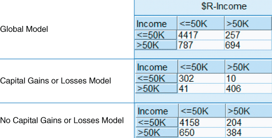
Figure 24.5 Contingency tables for Global Model and each Segmented Model.
Comparing the overall error rates,1 we have
Clearly, our segmentation models easily outperformed the global model. The overall error for the Caps Model was much lower, but the No Caps Model was also slightly lower. The combined model also saw a net 2.26 decrease in the overall error rate, which represents a better than 13% (0.0226/0.1696) decrease relative to the global model's error rate.
24.3 Segmentation Modeling using Clustering to Identify the Segments
The Churn data set is used to develop models to predict when customers will leave the company's service. We use clustering to develop segmentation models, in the hopes of better understanding the various segments of the company's clientele, using the following Cluster-Driven Segmentation Modeling Process for the Churn data set.
The cluster EDA is provided in Figure 24.6. The variables most helpful in discriminating between the clusters are shown at the top, in decreasing order of importance. Here, follow brief cluster profiles.
- Cluster 1. The No-Plan Majority. This cluster contains nearly 65% of the training set records (and a similar proportion of the test set). These customers belong to neither the International Plan nor the Voice Mail Plan.
- Cluster 2. The Voice Mail Plan People. This cluster contains about 25% of the records, and represents a preponderance of Voice Mail Plan users.
- Cluster 3. The International Plan People. This cluster contains only about 10% of the records, and represents those who have opted into the International Plan. Note that this cluster has a spike at the upper end of customer service calls, which does not bode well.
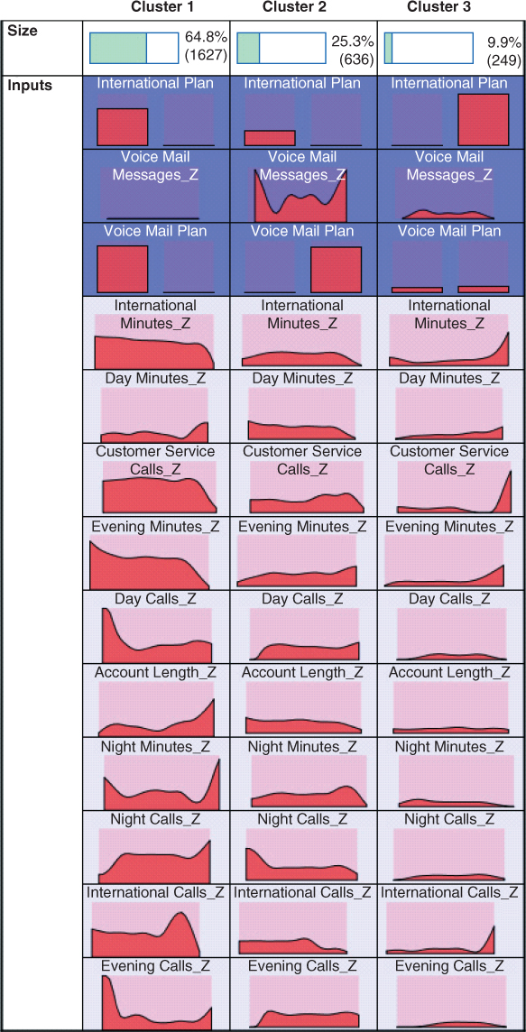
Figure 24.6 EDA for the clusters. Plan memberships are the most important variables for discriminating among the clusters.
Now, clearly, it is more expensive to get back a customer who has churned rather than to retain an existing customer. For this reason, in our CART models, we shall use a 2-to-1 misclassification cost for false negatives (i.e., predictions that actual churners will not churn).
The contingency tables for the Global Model and each of the cluster models are shown in Figure 24.7.
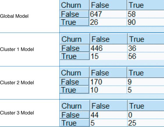
Figure 24.7 Contingency tables for the Global Model and each Cluster Model.
As we are using misclassification costs, then overall error rate is not as important as the model costs, as calculated here:
Thus, the combined costs of the cluster (segmentation) models (105) is about 4.5% less than the cost of the Global Model (110, units not specified), which should please your client. However, a further benefit of using clusters for segmentation is what the clusters reveal to us about the behavior of the customers. Figure 24.8 is a normalized bar graph of the clusters, with an overlay of churn (darker = true). Clearly, Cluster 3, the International Plan People, have a higher churn rate than the other two clusters. The company's managers should look to what is causing the adopters of the International Plan to leave the company's service.

Figure 24.8 Cluster 3 (International Plan People) has a higher churn rate.
From Figure 24.7 we can calculate the proportions of actual churners for each cluster, and for the entire test data set.
Cluster 3 has a much higher proportion of churners, than do the other clusters, as reflected in Figure 24.8.
Next, we can compare the decision trees built for each cluster, as shown in Figure 24.9. Note that the character of the decision trees for determining churn is distinct for each cluster, demonstrating the uniqueness of each segment, and calling for a customized approach by the company to alleviate customer churn for each segment.
- Cluster 1. The No-Plan Majority. The root node split is on Day Minutes_Z (standardized Day Minutes), with heavy users of day minutes (about 1.5 standard deviations above the mean) in danger of churning. Fortunately, there are not many of these. Otherwise, those with a large number of customer service calls (again, about 1.5 or more standard deviations above the mean, which works out to be at least four customer service calls) are at risk of churning.
- Cluster 2. The Voice Mail Plan People. Even though Cluster 2 has the lowest churn proportion among the clusters, we still need to be aware of those who are making a high number (at least four) of calls to customer service, for they are at a higher risk of churning. Note that the CART model shows that, even though only 38.9% of the 36 customers have a high number of calls to customer service, the prediction is still for Churn = True, because the misclassification cost of making a false negative error is twice as expensive.
- Cluster 3. The International Plan People. This is the cluster that is most troublesome to our company, with an over 40% churn rate. Clearly, our International service is driving customers away. The decision tree shows that International Plan members who do not make many International Calls
 have a 100% churn rate. Among the remaining customers, those with high International Minutes also have a 100% churn rate. Urgent intervention is called for to ameliorate these sad statistics.
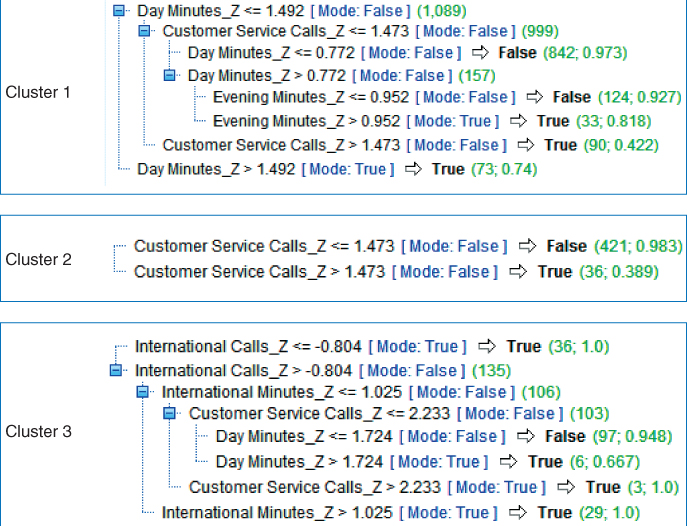
Figure 24.9 CART decision trees for each of the three clusters.
R References
- R Core Team. R: A Language and Environment for Statistical Computing. Vienna, Austria: R Foundation for Statistical Computing; 2012. ISBN: 3-900051-07-0, http://www.R-project.org/. Accessed 2014 Sep 30.
- Therneau T, Atkinson B, Ripley B. 2013. rpart: Recursive partitioning. R package version 4.1-3. http://CRAN.R-project.org/package=rpart.
Exercises
1. Give a thumbnail explanation of segmentation modeling.
2. Name two methods for identifying useful segments.
3. Explain the segmentation modeling process.
4. What would you say to a marketing manager who wished to use only one global model across his entire clientele, rather than trying segmentation models?
Hands-On Analysis
Use the WineQuality data set for Exercises 5–8.
5. Perform Z-standardization. Partition the data set into a training set and a test set.
6. Train a regression model to predict Quality using the entire training data set. This is our Global Model.
7. Evaluate the Global Model using the entire test data set, by applying the model generated on the training set to the records in the test set. Calculate the standard deviation of the errors (actual values − predicted values), and the mean absolute error. (For IBM/SPSS Modeler you can use the Analysis node to do this.)
8. Segment the training data set into red wines and white wines. Do the same for the test data set.
9. Train a regression model to predict Quality using the red wines in the training set. This is the Red Wines Model.
10. Train a regression model to predict Quality using the white wines in the training set. This is the White Wines Model.
11. Evaluate the Red Wines Model using the red wines from the test data set. Calculate the standard deviation of the errors, and the mean absolute error.
12. Evaluate the White Wines Model using the white wines from the test data set. Calculate the standard deviation of the errors, and the mean absolute error.
13. Compare the standard deviations of the errors, and the mean absolute errors, for the Global Model versus the combined results (weighted averages) from the Red Wines Model and the White Wines Model.
14. Contrast the regression models generated for the two types of wines. Discuss any substantive differences.