
Chapter 32
Case Study, Part 4: Modeling and Evaluation for High Performance Only
In this chapter, we are trading model interpretability for performance. We will take advantage of the fact that multicollinearity does not affect the model predictions, and not worry about substituting principal components for correlated predictors. In this way, as the set of original predictors contain more information than the set of principal components, we hope to develop models that will outperform those of Chapter 31, even while sacrificing interpretability.
32.1 Variables to be Input to the Models
The models in this chapter will benefit from a greater number of input variables, including many of the continuous variables that were subsumed into the principal components in Chapter 31. The listing of the variables is provided in Figure 32.1. Note that cluster membership remains an input, even though the principal components do not.

Figure 32.1 Listing of inputs to the models in this chapter.
32.2 Models that use Misclassification Costs
We begin using the two algorithms where we can specify our misclassification costs: classification and regression trees (CART) and C5.0. A CART model was trained on the training data set, and evaluated on the test data set. The contingency/costs table for the CART model is shown in Table 32.1, where the misclassification costs were specified as $1 for false positive, and $13.20 for false negative.
- Total cost for the CART model is
 .
. - Per customer cost for the CART model is
 .
.
Table 32.1 Contingency/costs table for the “performance CART model” with misclassification costs
| Predicted Category | |||
| Actual category | |||
So, the “CART performance model” beats the “Send to everyone” model by ![]() per customer. Further, the CART performance model beat the CART model from Chapter 31 by
per customer. Further, the CART performance model beat the CART model from Chapter 31 by ![]() to
to ![]() . The performance model did indeed outperform the earlier CART model using the principal components, at least in terms of estimated model cost.
. The performance model did indeed outperform the earlier CART model using the principal components, at least in terms of estimated model cost.
Next, a “performance C5.0 decision tree model” was run, with the misclassification costs given as $1 for false positive, and $13.20 for false negative. The contingency/costs table for the C5.0 model is shown in Table 32.2.
- Total cost for the C5.0 model is
 .
. - Per customer cost for the C5.0 model is
 .
.
Table 32.2 Contingency/costs table for the C5.0 model with misclassification costs
| Predicted Category | |||
| Actual category | |||
So, the performance C5.0 model beat the “Send to everyone” model by ![]() per customer. This performance C5.0 model did better than the C5.0 model from Chapter 31 that used the principal components, by
per customer. This performance C5.0 model did better than the C5.0 model from Chapter 31 that used the principal components, by ![]() to
to ![]() .
.
32.3 Models that Need Rebalancing as a Surrogate for Misclassification Costs
Next, in order to use rebalancing as a surrogate for misclassification costs for our neural networks and logistic regression models, we multiplied the number of records with positive responses in the training data set by the resampling ratio b = 13.2.
A “performance neural network model” was trained on the rebalanced training data set, and evaluated on the test data set, with the contingency/costs table shown in Table 32.3.
- Total cost for the neural network model is
 .
. - Per customer cost for the neural network model is
 .
.
Table 32.3 Contingency/costs table for the performance neural network model applied to the rebalanced data set
| Predicted Category | |||
| Actual category | |||
So, the neural network model beat the “Send to everyone” model by ![]() per customer. This performance neural network model scored better than the neural network model from Chapter 31 that used the principal components, by
per customer. This performance neural network model scored better than the neural network model from Chapter 31 that used the principal components, by ![]() to
to ![]() per customer.
per customer.
Finally, a “performance logistic regression model” was trained on the rebalanced training data set, and evaluated on the test data set, with the contingency/costs table shown in Table 32.4.
- Total cost for the logistic regression model is
 .
. - Per customer cost for the logistic regression model is
 .
.
Table 32.4 Contingency/costs table for the performance logistic regression model applied to the rebalanced data set
| Predicted Category | |||
| Actual category | |||
So, this logistic regression model beat the “Send to everyone” model by ![]() per customer. The performance logistic regression model also did better than the logistic regression model from Chapter 31 by
per customer. The performance logistic regression model also did better than the logistic regression model from Chapter 31 by ![]() .
.
32.4 Combining Models using Voting and Propensity Averaging
In Chapter 26, we learned how to combine models using model voting and propensity averaging. All of the “performance voting” combination models outperformed their counterparts from Chapter 31, but did not outperform the singleton performance neural network model above. Again, the threefold sufficient voting model had the best results among the voting models (Table 32.5). Propensity averaging was also applied, with similar results. The propensities of positive response for the four performance classification models were averaged, and a histogram of the resulting mean propensity is shown in Figure 32.2. A non-exhaustive search settled on the optimal cutoff to be mean propensity = 0.375, as shown in Table 32.5. This model predicts a positive response if the mean propensity to respond positively among the four models is 0.375 or greater. This model did well, but again did not outperform the singleton performance neural network model.
Table 32.5 Results from combining performance models using voting and propensity averaging (best performance highlighted)
| Model | Total Model Profit | Profit per Customer |
| “Send to All” model | $18 596.40 | $2.59 |
| CART model | |
|
| C5.0 model | |
|
| Neural network | |
|
| Logistic regression | |
|
| Single sufficient | $23 653.60 | $3.29 |
| Twofold sufficient | $24 136.40 | $3.35 |
| Threefold sufficient | $24 223.60 | $3.37 |
| Positive unanimity | 23,895.2 | $3.32 |
| Mean propensity 0.374 | $24 224.80 | $3.37 |
| Mean propensity 0.375 | $24 236.80 | $3.37 |
| Mean propensity 0.376 | $24 198.00 | $3.37 |
For clarity, profit rather than cost is listed, where profit = –cost. For completeness, the results from the singleton models are included as well.
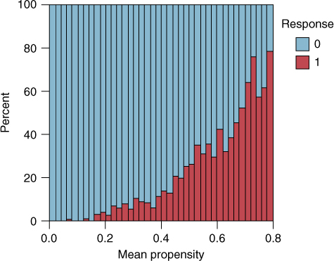
Figure 32.2 Mean propensity, with response overlay.
Again, the reader is invited to try further model enhancements, if desired, such as the use of segmentation modeling, and boosting and bagging.
32.5 Lessons Learned
Clearly, the “performance” models in this chapter outperform the models in Chapter 31, which use the principal components. The average improvement in profit across the models in Table 32.5 over their counterparts in Chapter 31 is about ![]() . Allowing the models to use the actual predictors rather than the principal components led to this increase in profitability. In other words, more information leads to better models.
. Allowing the models to use the actual predictors rather than the principal components led to this increase in profitability. In other words, more information leads to better models.
The downside of the performance models is lack of interpretability. It is symbolic here that the most profitable performance model is the neural network model, which is well-known for its lack of interpretability in any case. Where the neural network shines is when there are nonlinear associations in the data, which other types of models have difficulty in sifting through. This evidently is the situation in our clothing store data.
32.6 Conclusions
So, in the end, have we addressed our primary and secondary objectives?
- Primary Objective: Develop a classification model that will maximize profits for direct mail marketing.
- Secondary Objective: Develop better understanding of our clientele through EDA, component profiles, and cluster profiles.
In chapter 29, 30, and 31, we developed a much better understanding of our clientele, using exploratory data analysis, component profiles, cluster profiles, and interpretation of the best performing model in Chapter 31. In chapter 31 and 32, we have developed a set of models that will make a good bit of money for our clothing store company, to the tune of $3.46 per customer, an increase of $0.87 per customer over the “Send to everyone” model the company was probably using before the lessons learned from the Case Study a 25% increase in profits. In thus fulfilling the primary and secondary objectives for this Case Study, the predictive analyst has rendered valuable service, by leveraging existing data to enhance knowledge and profitability.