
Chapter 25
Ensemble Methods: Bagging and Boosting
Here in Part 6: Enhancing Model Performance, we are learning methods that allow us to improve the performance of our models. In Chapter 24 we learned about Segmentation Models, where a useful clustering or subdivision of the data set is found, allowing us to develop cluster-specific models for each segment, and thereby enhancing the overall efficacy of the classification task. Here in this chapter, we are introduced to Ensemble Methods, specifically, bagging and boosting that combine the results from a set of classification models (classifiers), in order to increase the accuracy and reduce the variability of the classification. Next time, in Chapter 26, we consider other types of ensemble methods, including voting and model averaging.
We have become acquainted with a wide range of classification algorithms in this book, including
- k-nearest neighbor classification
- Classification and regression trees (CART)
- The C4.5 algorithm
- Neural networks for classification
- Logistic regression
- Naïve Bayes and Bayesian networks.
However, we have so far used our classification algorithms one at a time. Have you wondered what would happen if we were somehow able to combine more than one classification model? Might the resulting combined model be more accurate, or have less variability?
What would be the rationale for using an ensemble of classification models?
25.1 Rationale for Using an Ensemble of Classification Models
The benefits of using an ensemble of classification models rather than a single classification model are that
- the ensemble classifier is likely to have a lower error rate (boosting);
- the variance of the ensemble classifier will be lower than had we used certain unstable classification models, such as decision trees and neural networks, that have high variability (bagging and boosting);
How does an ensemble classifier succeed in having a lower error rate than the single classifier? Consider the following example.
Suppose we have an ensemble of five binary (0/1, yes/no) classifiers, each of which has an error rate of 0.20. The ensemble classifier will consider the classification (prediction) for each classifier, and the classification with the most votes among the five classifiers will be chosen as the output class for the ensemble classifier. If the individual classifiers classify the cases similarly, then the ensemble classifier will follow suit, in which case the error rate for the ensemble method will be the same as for the individual classifiers, 0.20.
However, if the individual classifiers are independent, that is, if the classification errors of the individual classifiers are uncorrelated, then the voting mechanism ensures that the ensemble classifier will make an error only when the majority of individual classifiers make an error. We may calculate the error rate of the ensemble classifier in this case using the binomial probability distribution formula.
Let ![]() represent the individual classifier error rate. The probability that
represent the individual classifier error rate. The probability that ![]() of the five individual classifiers will make the wrong prediction is
of the five individual classifiers will make the wrong prediction is
So, the probability that three of the five classifiers will make an error is
Similarly, the probability that four of the individual classifiers will make a wrong prediction is
And the probability that all five of the classifiers will make an error is
Thus, the error rate of the ensemble classifier in this case equals:
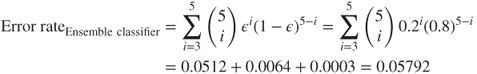
which is much lower than the base error rate of the individual classification models, 0.20.
When the base error rate is greater than 0.5, however, combining independent models into an ensemble classifier will lead to an even greater error rate. An exercise in this section asks the reader to demonstrate how this is the case. Here in Chapter 25, we examine two ensemble methods for improving classification model performance: bagging and boosting. But first, we need to consider how the efficacy of a prediction model is measured.
25.2 Bias, Variance, and Noise
We would like our models, either estimation models or classification models, to have low prediction error. That is, we would like the distance ![]() between our target
between our target ![]() and our prediction
and our prediction ![]() to be small. The prediction error for a particular observation can be decomposed as follows:
to be small. The prediction error for a particular observation can be decomposed as follows:
where
- Bias refers to the average distance between the predictions (
 , represented by the lightning darts in Figure 25.1) and the target (y, the bull's eye);
 - Variance measures the variability in the predictions
 themselves;
 - Noise represents the lower bound on the prediction error that the predictor can possibly achieve.
To reduce the prediction error, then, we need to reduce the bias, the variance, or the noise. Unfortunately, there is nothing we can do to reduce the noise: It is an intrinsic characteristic of the prediction problem. Thus, we must try to reduce either the bias or the variance. As we shall see, bagging can reduce the variance of classifier models, while boosting can reduce both bias and variance. Thus, boosting offers a way to short-circuit the bias–variance trade-off,a where efforts to reduce bias will necessarily increase the variance, and vice versa.


25.3 When to Apply, and not to apply, Bagging
Neural networks models can often fit a model to the available training data quite well, so that they have low bias. However, small changes in initial conditions can lead to high variability in predictions, so that neural networks are considered to have low bias but high variance. This high variability would qualify neural networks as an unstable classifier. According to Leo Breiman.
Some classification and regression methods are unstable in the sense that small perturbations in their training sets or in construction may result in large changes in the constructed predictor.Reference: Arcing Classifiers, by Leo Breiman, The Annals of Statistics, Vol 26, No. 3, 801–849, 1998
Table 25.1 contains a listing of the classification algorithms that Breiman states are either stable or unstable.
Table 25.1 Stable or unstable classification algorithms
| Classification Algorithm | Stable or Unstable |
| Classification and regression trees | Unstable |
| C4.5 | Unstable |
| Neural networks | Unstable |
| k-Nearest neighbor | Stable |
| Discriminant analysis | Stable |
| Naïve bayes | Stable |
It would make sense that a method for reducing variance would work best with unstable models, where there is room for improvement in reducing variability. Thus, it is with bagging, which works best with unstable models such as neural networks. It is worthwhile to apply bagging to unstable models, but applying bagging to stable models can degrade their performance. This is because bagging works with bootstrap samples of the original data, each of which contains only about 63% of the data (see below). Thus, it is unwise to apply bagging to k-nearest neighbor models or other stable classifiers.
25.4 Bagging
The term bagging was coined by Leo Breimanb to refer to Bootstrap Aggregating; the bagging algorithm is shown here.
Thus, the bootstrap samples are drawn in Step 1, the base models are trained in Step 2, and the results are aggregated in Step 3. Note that this process of aggregation, either by voting or by taking the average, has the effect (for unstable models) of reducing the error due to model variance. The reduction in variance accomplished by bagging is in part due to the averaging out of nuisance outliers that will occur in some of the bootstrap samples, but not others.
By way of analogy, consider a normal population with mean ![]() and variance
and variance ![]() . The sample mean
. The sample mean ![]() , representing the aggregation, will then be distributed as normal, with mean
, representing the aggregation, will then be distributed as normal, with mean ![]() and variance
and variance ![]() , for sample size
, for sample size ![]() . That is, the variance of the aggregated statistic
. That is, the variance of the aggregated statistic ![]() is smaller than that of an individual observation
is smaller than that of an individual observation ![]() .
.
Because sampling with replacement is used, certain observations will occur more than once in a particular bootstrap sample, while others will not occur at all. It can be shown that a bootstrap sample contains about 63% of the records in the original training data set. This is because each observation has the following probability of being selected for a bootstrap sample:
and, for sufficiently large n, this converges to
This is why the performance of stable classifiers like ![]() -nearest neighbor may be degraded by using bagging, as the bootstrap samples are each missing on average 37% of the original data.
-nearest neighbor may be degraded by using bagging, as the bootstrap samples are each missing on average 37% of the original data.
To see how bagging works, consider the data set in Table 25.2. Here, ![]() denotes the variable value and
denotes the variable value and ![]() denotes the classification, either 0 or 1. Suppose we have a one-level decision tree classifier that chooses a value of
denotes the classification, either 0 or 1. Suppose we have a one-level decision tree classifier that chooses a value of ![]() that will minimize leaf node entropy for the test condition
that will minimize leaf node entropy for the test condition ![]() .
.
Table 25.2 Data set to be sampled to create the bootstrap samples
| x | 0.2 | 0.4 | 0.6 | 0.8 | 1 |
| y | 1 | 0 | 0 | 0 | 1 |
Now, if bagging is not used, then the best that our classifier can do is to split at ![]() or
or ![]() , resulting in either cases with 20% error rate. However, suppose we now apply the bagging algorithm.
, resulting in either cases with 20% error rate. However, suppose we now apply the bagging algorithm.
Step 1 Bootstrap samples are taken with replacement for the data set in Table 25.2. These samples are shown in Table 25.3. (Of course, your bootstrap samples will differ.)
-
Table 25.3 Bootstrap samples drawn from Table 25.2, with the base classifiers
Bootstrap Sample Base Classifier 1 x 0.2 0.2 0.4 0.6 1 
y 1 1 0 0 1 
2 x 0.2 0.4 0.4 0.6 0.8 
y 1 0 0 0 0 
3 x 0.4 0.4 0.6 0.8 1 
y 0 0 0 0 1 
4 x 0.2 0.6 0.8 1 1 
y 1 0 0 1 1 
5 x 0.2 0.2 1 1 1 
y 1 1 1 1 1 
Table 25.4 Collection of predictions of base classifiers
Bootstrap Sample 


1 1 0 0 0 0 2 1 0 0 0 0 3 0 0 0 0 1 4 0 0 0 0 1 5 1 1 1 1 1 Proportion 0.6 0.2 0.2 0.2 0.6 Bagging prediction 1 0 0 0 1 Proportion of 1's = average ⇒ majority bagging prediction.
- Step 2 The one-level decision tree classifiers (base classifiers) are trained on each separate sample, and shown on the right side of Table 25.3.
- Step 3 For each record, the votes are tallied, and the majority class is selected as the decision of the bagging ensemble classifier. As we have a 0/1 classification, this majority equals the average of the individual classifiers, the proportion of 1's. If the proportion is less than 0.5, then the bagging prediction is 0, otherwise 1. The proportions and bagging predictions are shown in Table 25.4.
In this case, the bagging prediction classifies each record correctly, so that the error rate is zero for this toy example. Of course, in most big data applications, this does not occur.
Breiman states, “The vital element is the instability of the prediction method.” If the base classifier is unstable, then bagging can contribute to a reduction in the prediction error, because it reduces the classifier variance without affecting the bias, and recall that Prediction error = Bias + Variance + Noise. If, however, the base classifier is stable, then the prediction error stems mainly from the bias in the base classifier; so applying bagging will not help, and may even degrade performance, because each bootstrap sample contains on an average only 63% of the data. Usually, however, bagging is used to reduce the classifier variability for unstable base classifiers, and thus the bagging ensemble model will exhibit enhanced generalizability to the test data.
Bagging does have a downside. The beauty of decision trees, which because of their instability are common candidates for bagging, is their simplicity and interpretability. Clients can understand the flow of a decision tree, and the factors leading to a particular classification. However, aggregating (by voting or averaging) a set of decision trees obfuscates the simple structure of the base decision tree, and loses the easy interpretability.
For stable base classifiers, an alternative strategy is to take bootstrap samples of the predictors rather than the records. This may be especially fruitful when there are sets of highly correlated predictors.c
25.5 Boosting
Boosting was developed by Freund and Schapire in the 1990s.d Boosting differs from bagging in that the algorithm is adaptive. The same classification model is applied successively to the training sample, except that, in each iteration, the boosting algorithm applies greater weight to the records that have been misclassified. Boosting has the double benefit of reducing the error due to variance (such as bagging) and also due to bias.
Here follows a toy example of the ADABoost boosting algorithm, first published in the book Boosting: Foundations and Algorithms, by Robert E. Schapire and Yoav Freund.e
Step 1 The original training data set ![]() consists of a set of 10 dichotomous values, as shown in Figure 25.2. An initial base classifier
consists of a set of 10 dichotomous values, as shown in Figure 25.2. An initial base classifier ![]() is determined to separate the two leftmost values from the others (Figure 25.3). Shaded area represents values classified as “+.”
is determined to separate the two leftmost values from the others (Figure 25.3). Shaded area represents values classified as “+.”
-
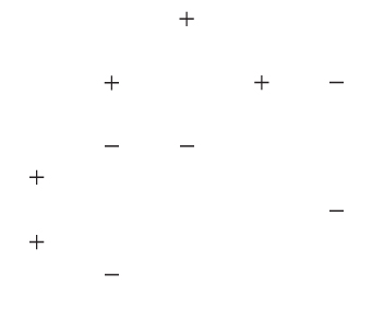
Figure 25.2 Original data.

Figure 25.3 Initial base classifier.
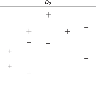
Figure 25.4 First reweighting of the data.

Figure 25.5 Second base classifier.
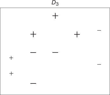
Figure 25.6 Second reweighting of the data.

Figure 25.7 Third base classifier.
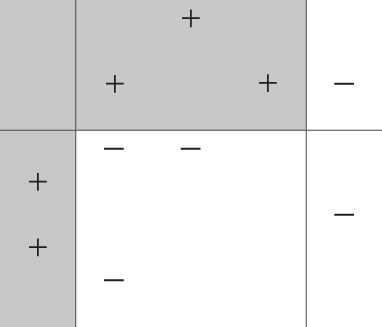
Figure 25.8 Final boosted classifier is a weighted average of the three base classifiers.
- Step 2 (First pass.) There were three values incorrectly classified by
 , as shown by the boxed “+” signs in Figure 25.3. These three values have their weights (represented by their relative size in the diagrams) increased, while the other seven values have their weights decreased. This new data distribution
  is shown in Figure 25.4. Based on the new weights in
  , a new base classifier
  is determined, as shown in Figure 25.5.
 - Step 2 (Second pass.) Three values incorrectly classified by
 , as shown by the boxed “−” signs in Figure 25.5. These three values have their weights (represented by their relative size in the diagrams) increased, while the other seven values have their weights decreased. This new data distribution
  is shown in Figure 25.6. Based on the new weights in
  , a new base classifier
  is determined, as shown in Figure 25.7.
 - Step 3 The final boosted classifier, shown in Figure 25.8, is the weighted sum of the
 base classifiers:
  .
.
The weights ![]() assigned to each base classifier are proportional to the accuracy of the classifier. For details on how the actual weights are calculated, see the book by Schapire and Freund. Just as for bagging, boosting performs best when the base classifiers are unstable. By focusing on classification errors, boosting has the effect of reducing both the error due to bias and the error due to variance. However, boosting can increase the variance when the base classifier is stable. Also, boosting, such as bagging, obfuscates the interpretability of the results.
assigned to each base classifier are proportional to the accuracy of the classifier. For details on how the actual weights are calculated, see the book by Schapire and Freund. Just as for bagging, boosting performs best when the base classifiers are unstable. By focusing on classification errors, boosting has the effect of reducing both the error due to bias and the error due to variance. However, boosting can increase the variance when the base classifier is stable. Also, boosting, such as bagging, obfuscates the interpretability of the results.
25.6 Application of Bagging and Boosting Using IBM/SPSS Modeler
Finally, we offer an example of the efficacy of bagging and boosting for reducing prediction error. The ClassifyRisk data set was partitioned into training and test data sets, and three models were developed using the training set: (i) an original CART model for predicting risk, (ii) a bagging model, where five base models were sampled with replacement from the training set, and (iii) a boosting model, where five iterations of the boosting algorithm were applied.
Each of (i), (ii), and (iii) were then applied to the unseen test data set. The resulting contingency tables are shown in Figure 25.9, where the predicted risk (“$R-risk”) is given in the columns and the actual risk is given in the rows. A comparison of the error rates shows that the error rates for the bagging and boosting models are lower than that of the original CART model.f

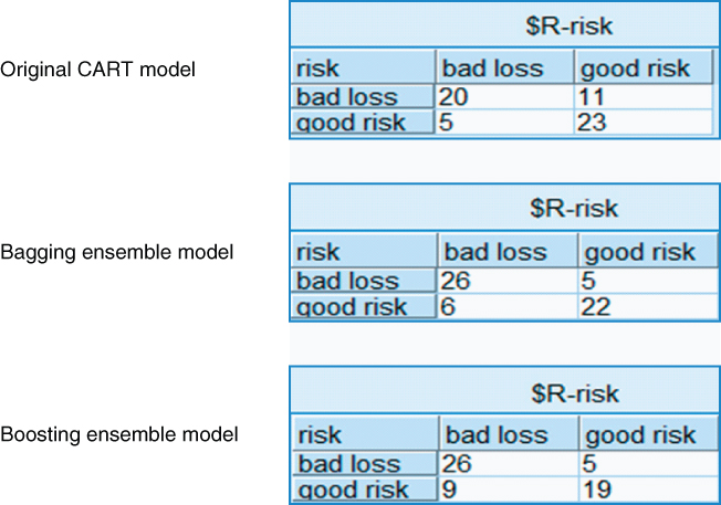
Figure 25.9 Ensemble models have lower error rates than the original CART model.
Unfortunately, these lower error rates come with a loss of easy interpretability. Figure 25.10 shows the decision tree for the original CART model. From this tree, the client could implement any number of actionable decision rules, such as, for example, “If customer income ≤$37,786.33 and age ≤47.5 and marital status is single or other, then we predict a bad loss, with 97.6% confidence.” The ensemble methods lose this ease of interpretability by aggregating the results of several decision trees.
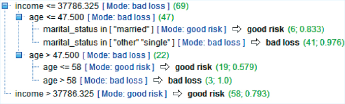
Figure 25.10 Decision tree for Original CART model offers greater interpretability.
References
Apart from the sources referenced above, the following books have excellent treatment of ensemble methods, including bagging and boosting.
- Introduction to Data Mining, by Pang-Ning Tan, Michael Steinbach, and Vipin Kumar, Pearson Education, 2006.
- Data Mining for Statistics and Decision Making, by Stephane Tuffery, John Wiley and Sons, 2011.
R Reference
- 1. R Core Team. R: A Language and Environment for Statistical Computing. Vienna, Austria: R Foundation for Statistical Computing; 2012. 3-900051-07-0, http://www.R-project.org/. Accessed 01 Oct 2014.
Exercises
1. Describe two benefits of using an ensemble of classification models.
2. Recall the example at the beginning of the chapter, where we show that an ensemble of five independent binary classifiers has a lower error rate than the base error rate of 0.20. Demonstrate that an ensemble of three independent binary classifiers, each of which has a base error rate of 0.10, has a lower error rate than 0.10.
3. Demonstrate that an ensemble of five independent binary classifiers, each with a base error rate of 0.6, has a higher error rate than 0.6.
4. What is the equation for the decomposition of the prediction error?
5. Explain what is meant by the following terms: bias, variance, and noise.
6. True or false: bagging can reduce the variance of classifier models, while boosting can reduce both bias and variance.
7. What does it mean for a classification algorithm to be unstable?
8. Which classification algorithms are considered unstable? Which are considered stable?
9. What can happen if we apply bagging to stable models? Why might this happen?
10. What is a bootstrap sample?
11. State the three steps of the bagging algorithm.
12. How does bagging contribute to a reduction in the prediction error?
13. What is a downside of using bagging?
14. State the three steps of the boosting algorithm.
15. Explain what we mean when we say that the boosting algorithm is adaptive.
16. Does the boosting algorithm use bootstrap samples?
17. The boosting algorithm uses a weighted average of a series of classifiers. On what do the weights in this weighted average depend?
18. True or false: Unlike bagging, boosting does not suffer from a loss of interpretability of the results.
Use the following information for Exercises 19–23. Table 25.5 represents the data set to be sampled to create bootstrap samples. Five bootstrap samples are shown in Table 25.6.
Table 25.5 Data set to be sampled to create the bootstrap samples
| x | 0 | 0.5 | 1 |
| y | 1 | 0 | 1 |
Table 25.6 Bootstrap samples drawn from Table 25.5
| Bootstrap Sample | ||||
| 1 | x | 0 | 0 | 0.5 |
| y | 1 | 1 | 0 | |
| 2 | x | 0.5 | 1 | 1 |
| y | 0 | 1 | 1 | |
| 3 | x | 0 | 0 | 1 |
| y | 1 | 1 | 1 | |
| 4 | x | 0.5 | 0.5 | 1 |
| y | 0 | 0 | 1 | |
| 5 | x | 0 | 0.5 | 0.5 |
| y | 1 | 0 | 0 | |
19. Construct the base classifier for each bootstrap sample, analogous to those found in Table 25.3.
20. Provide a table of the predictions for each base classifier, similarly to those found in Table 25.4.
21. Find the proportion of 1's, and make the majority prediction for each value of x, similarly to that in Table 25.4.
22. Verify that the ensemble classifier correctly predicts the three values of x.
23. Change the fifth bootstrap sample in Table 25.6 to the following:
| x | 0.5 | 0.5 | 1 |
| y | 0 | 0 | 1 |
Recalculate the proportion of 1's, and the majority predictions for each value of x. Conclude that the bagging classifier does not always correctly predict all values of x.
Hands-On Analysis
Use the ClassifyRisk data set for Exercises 24–27.
24. Partition the data set into training and test data sets.
25. Develop three models using the training data set: (i) an original CART model for predicting risk, (ii) a bagging model, where five base models are sampled with replacement from the training set, and (iii) a boosting model, where five iterations of the boosting algorithm are applied.
26. Apply each of (i), (ii), and (iii) to the test data set. Produce the contingency tables for each model. Compare the error rates for the bagging and boosting models against that of the original CART model.
27. Extract a sample interesting decision rule from the original CART model. Comment on the interpretability of the results from the bagging and boosting models.