
Chapter 7
Preparing to Model the Data
7.1 Supervised Versus Unsupervised Methods
Data mining methods may be categorized as either supervised or unsupervised. In unsupervised methods, no target variable is identified as such. Instead, the data mining algorithm searches for patterns and structures among all the variables. The most common unsupervised data mining method is clustering, our topic for Chapters 19–22. For example, political consultants may analyze congressional districts using clustering methods, to uncover the locations of voter clusters that may be responsive to a particular candidate's message. In this case, all appropriate variables (e.g., income, race, gender) would be input to the clustering algorithm, with no target variable specified, in order to develop accurate voter profiles for fund-raising and advertising purposes.
Another data mining method, which may be supervised or unsupervised, is association rule mining. In market basket analysis, for example, one may simply be interested in “which items are purchased together,” in which case no target variable would be identified. The problem here, of course, is that there are so many items for sale, that searching for all possible associations may present a daunting task, due to the resulting combinatorial explosion. Nevertheless, certain algorithms, such as the a priori algorithm, attack this problem cleverly, as we shall see when we cover association rule mining in Chapter 23.
Most data mining methods are supervised methods, however, meaning that (i) there is a particular prespecified target variable, and (ii) the algorithm is given many examples where the value of the target variable is provided, so that the algorithm may learn which values of the target variable are associated with which values of the predictor variables. For example, the regression methods of Chapters 8 and 9 are supervised methods, as the observed values of the response variable y are provided to the least-squares algorithm, which seeks to minimize the squared distance between these y values and the y values predicted given the x-vector. All of the classification methods we examine in Chapters 10–18 are supervised methods, including decision trees, neural networks, and k-nearest neighbors.
Note: The terms supervised and unsupervised are widespread in the literature, and hence used here. However, we do not mean to imply that unsupervised methods require no human involvement. To the contrary, effective cluster analysis and association rule mining both require substantial human judgment and skill.
7.2 Statistical Methodology and Data Mining Methodology
In Chapters 5 and 6, we were introduced to a wealth of statistical methods for performing inference, that is, for estimating or testing the unknown parameters of a population of interest. Statistical methodology and data mining methodology differ in the following two ways:
- Applying statistical inference using the huge sample sizes encountered in data mining tends to result in statistical significance, even when the results are not of practical significance.
- In statistical methodology, the data analyst has an a priori hypothesis in mind. Data mining procedures usually do not have an a priori hypothesis, instead freely trolling through the data for actionable results.
7.3 Cross-Validation
Unless properly conducted, data mining can become data dredging, whereby the analyst “uncovers” phantom spurious results, due to random variation rather than real effects. It is therefore crucial that data miners avoid data dredging. This is accomplished through cross-validation.
Cross-validation is a technique for insuring that the results uncovered in an analysis are generalizable to an independent, unseen, data set. In data mining, the most common methods are twofold cross-validation and k-fold cross-validation. In twofold cross-validation, the data are partitioned, using random assignment, into a training data set and a test data set. The test data set should then have the target variable omitted. Thus, the only systematic difference between the training data set and the test data set is that the training data includes the target variable and the test data does not. For example, if we are interested in classifying income bracket, based on age, gender, and occupation, our classification algorithm would need a large pool of records, containing complete (as complete as possible) information about every field, including the target field, income bracket. In other words, the records in the training set need to be preclassified. A provisional data mining model is then constructed using the training samples provided in the training data set.
However, the training set is necessarily incomplete; that is, it does not include the “new” or future data that the data modelers are really interested in classifying. Therefore, the algorithm needs to guard against “memorizing” the training set and blindly applying all patterns found in the training set to the future data. For example, it may happen that all customers named “David” in a training set may be in the high-income bracket. We would presumably not want our final model, to be applied to the new data, to include the pattern “If the customer's first name is David, the customer has a high income.” Such a pattern is a spurious artifact of the training set and needs to be verified before deployment.
Therefore, the next step in supervised data mining methodology is to examine how the provisional data mining model performs on a test set of data. In the test set, a holdout data set, the values of the target variable are hidden temporarily from the provisional model, which then performs classification according to the patterns and structures it learned from the training set. The efficacy of the classifications is then evaluated by comparing them against the true values of the target variable. The provisional data mining model is then adjusted to minimize the error rate on the test set.
Estimates of model performance for future, unseen data can then be computed by observing various evaluative measures applied to the test data set. Such model evaluation techniques are covered in Chapters 15–18. The bottom line is that cross-validation guards against spurious results, as it is highly unlikely that the same random variation would be found to be significant in both the training set and the test set. For example, a spurious signal with 0.05 probability of being observed, if in fact no real signal existed, would have only ![]() probability of being observed in both the training and test sets, because these data sets are independent. In other words, the data analyst could report an average 400 results before one would expect a spurious result to be reported.
probability of being observed in both the training and test sets, because these data sets are independent. In other words, the data analyst could report an average 400 results before one would expect a spurious result to be reported.
But the data analyst must insure that the training and test data sets are indeed independent, by validating the partition. We validate the partition into training and test data sets by performing graphical and statistical comparisons between the two sets. For example, we may find that, even though the assignment of records was made randomly, a significantly higher proportion of positive values of an important flag variable were assigned to the training set, compared to the test set. This would bias our results, and hurt our prediction or classification accuracy on the test data set. It is especially important that the characteristics of the target variable be as similar as possible between the training and test data sets. Table 7.1 shows the suggested hypothesis test for validating the target variable, based on the type of target variable.
Table 7.1 Suggested hypothesis tests for validating different types of target variables
| Type of Target Variable | Test from Chapter 5 |
| Continuous | Two-sample t-test for difference in means |
| Flag | Two-sample Z test for difference in proportions |
| Multinomial | Test for homogeneity of proportions |
In k-fold cross validation, the original data is partitioned into k independent and similar subsets. The model is then built using the data from k − 1 subsets, using the kth subset as the test set. This is done iteratively until we have k different models. The results from the k models are then combined using averaging or voting. A popular choice for k is 10. A benefit of using k-fold cross-validation is that each record appears in the test set exactly once; a drawback is that the requisite validation task is made more difficult.
To summarize, most supervised data mining methods apply the following methodology for building and evaluating a model:
7.4 Overfitting
Usually, the accuracy of the provisional model is not as high on the test set as it is on the training set, often because the provisional model is overfitting on the training set. Overfitting results when the provisional model tries to account for every possible trend or structure in the training set, even idiosyncratic ones such as the “David” example above. There is an eternal tension in model building between model complexity (resulting in high accuracy on the training set) and generalizability to the test and validation sets. Increasing the complexity of the model in order to increase the accuracy on the training set eventually and inevitably leads to a degradation in the generalizability of the provisional model to the test set, as shown in Figure 7.1.
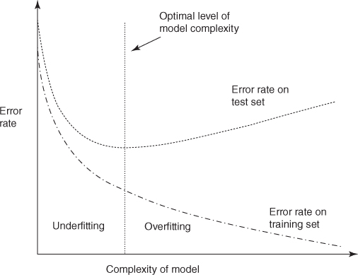
Figure 7.1 The optimal level of model complexity is at the minimum error rate on the test set.
Figure 7.1 shows that as the provisional model begins to grow in complexity from the null model (with little or no complexity), the error rates on both the training set and the test set fall. As the model complexity increases, the error rate on the training set continues to fall in a monotone manner. However, as the model complexity increases, the test set error rate soon begins to flatten out and increase because the provisional model has memorized the training set rather than leaving room for generalizing to unseen data. The point where the minimal error rate on the test set is encountered is the optimal level of model complexity, as indicated in Figure 7.1. Complexity greater than this is considered to be overfitting; complexity less than this is considered to be underfitting.
7.5 Bias–Variance Trade-Off
Suppose that we have the scatter plot in Figure 7.2 and are interested in constructing the optimal curve (or straight line) that will separate the dark gray points from the light gray points. The straight line has the benefit of low complexity but suffers from some classification errors (points ending up on the wrong side of the line).

Figure 7.2 Low-complexity separator with high error rate.
In Figure 7.3, we have reduced the classification error to zero but at the cost of a much more complex separation function (the curvy line). One might be tempted to adopt the greater complexity in order to reduce the error rate. However, one should be careful not to depend on the idiosyncrasies of the training set. For example, suppose that we now add more data points to the scatter plot, giving us the graph in Figure 7.4.

Figure 7.3 High-complexity separator with low error rate.

Figure 7.4 With more data: low-complexity separator need not change much; high-complexity separator needs much revision.
Note that the low-complexity separator (the straight line) need not change very much to accommodate the new data points. This means that this low-complexity separator has low variance. However, the high-complexity separator, the curvy line, must alter considerably if it is to maintain its pristine error rate. This high degree of change indicates that the high-complexity separator has a high variance.
Even though the high-complexity model has a low bias (in terms of the error rate on the training set), it has a high variance; and even though the low-complexity model has a high bias, it has a low variance. This is what is known as the bias–variance trade-off. The bias–variance trade-off is another way of describing the overfitting/underfitting dilemma shown in Figure 7.1. As model complexity increases, the bias on the training set decreases but the variance increases. The goal is to construct a model in which neither the bias nor the variance is too high, but usually, minimizing one tends to increase the other.
For example, a common method of evaluating how accurate model estimation is proceeding for a continuous target variable is to use the mean-squared error (MSE). Between two competing models, one may select the better model as that model with the lower MSE. Why is MSE such a good evaluative measure? Because it combines both bias and variance. The MSE is a function of the estimation error (sum of squared errors, SSE) and the model complexity (e.g., degrees of freedom). It can be shown (e.g., Hand, Mannila, and Smyth.1) that the MSE can be partitioned using the following equation, which clearly indicates the complementary relationship between bias and variance:
7.6 Balancing The Training Data Set
For classification models, in which one of the target variable classes has much lower relative frequency than the other classes, balancing is recommended. A benefit of balancing the data is to provide the classification algorithms with a rich balance of records for each classification outcome, so that the algorithms have a chance to learn about all types of records, not just those with high target frequency. For example, suppose we are running a fraud classification model and our training data set consists of 100,000 transactions, of which only 1000 are fraudulent. Then, our classification model could simply predict “non-fraudulent” for all transactions, and achieve 99% classification accuracy. However, clearly this model is useless.
Instead, the analyst should balance the training data set so that the relative frequency of fraudulent transactions is increased. There are two ways to accomplish this, which are as follows:
- Resample a number of fraudulent (rare) records.
- Set aside a number of non-fraudulent (non-rare) records.
Resampling refers to the process of sampling at random and with replacement from a data set. Suppose we wished our 1000 fraudulent records to represent 25% of the balanced training set, rather than the 1% represented by these records in the raw training data set. Then, we could add 32,000 resampled fraudulent records so that we had 33,000 fraudulent records, out of a total of 100,000 + 32,000 = 132,000 records in all. This represents ![]() or the desired 25%.
or the desired 25%.
How did we arrive at the number of 32,000 additional fraudulent records? By using the equation
and solving for x, the required number of additional records to resample. In general, this equation is
and solving for x gives us:
where x is the required number of resampled records, p represents the desired proportion of rare values in the balanced data set, records represents the number of records in the unbalanced data set, and rare represents the current number of rare target values.
Some data miners have a philosophical aversion to resampling records to achieve balance, as they feel this amounts to fabricating data. In this case, a sufficient number of non-fraudulent transactions would instead be set aside, thereby increasing the proportion of fraudulent transactions. To achieve a 25% balance proportion, we would retain only 3000 non-fraudulent records. We would then need to discard from the analysis 96,000 of the 99,000 non-fraudulent records, using random selection. It would not be surprising if our data mining models would suffer as a result of starving them of data in this way. Instead, the data analyst would probably be well-advised either to decrease the desired balance proportion to something like 10% or to use resampling.
When choosing a desired balancing proportion, recall the rationale for doing so: in order to allow the model a sufficiently rich variety of records to learn how to classify the rarer value of the target variable across a range of situations. The balancing proportion can be relatively low (e.g., 10%) if the analyst is confident that the rare target value is exposed to a sufficiently rich variety of records. The balancing proportion should be higher (e.g., 25%) if the analyst is not so confident of this.
The test data set should never be balanced. The test data set represents new data that the models have not seen yet. Certainly, the real world will not balance tomorrow's data for the convenience of our classification models; therefore, the test data set itself should not be balanced. Note that all model evaluation will take place using the test data set, so that the evaluative measures will all be applied to unbalanced (real-world-like) data.
Because some predictor variables have higher correlation with the target variable than do other predictor variables, the character of the balanced data will change. For example, suppose we are working with the Churn data set, and suppose that churners have higher levels of day minutes than non-churners. Then, when we balance the data set, the overall mean of day minutes will increase, as we have eliminated so many non-churner records. Such changes cannot be avoided when balancing data sets. Thus, direct overall comparisons between the original and balanced data sets are futile, as changes in character are inevitable. However, apart from these unavoidable changes, and although the random sampling tends to protect against systematic deviations, data analysts should provide evidence that their balanced data sets do not otherwise differ systematically from the original data set. This can be accomplished by examining the graphics and summary statistics from the original and balanced data set, partitioned on the categories of the target variable. If desired, hypothesis tests such as those in Chapter 6 may be applied. If deviations are uncovered, the balancing should be reapplied. Cross-validation measures can be applied if the analyst is concerned about these deviations. Multiple randomly selected balanced data sets can be formed, and the results averaged, for example.
7.7 Establishing Baseline Performance
In Star Trek IV: The Voyage Home, Captain Kirk travels back in time to the 20th century, finds himself in need of cash, and pawns his eyeglasses. The buyer offers him $100, to which Captain Kirk responds, “Is that a lot?” Unfortunately, the Captain had no frame of reference to compare the $100 to, and so was unable to determine whether the $100 was a satisfactory offer or not. As data analysts we should do our best to avoid putting our clients into Captain Kirk's situation, by reporting results with no comparison to a baseline. Without comparison to a baseline, a client cannot determine whether our results are any good.
For example, suppose we naively report that “only” 28.4% of customers adopting our International Plan (see Table 3.3) will churn. That does not sound too bad, until we recall that, among all of our customers, the overall churn rate is only 14.49% (Figure 3.3). This overall churn rate may be considered our baseline, against which any further results can be calibrated. Thus, belonging to the International Plan actually nearly doubles the churn rate, which is clearly not good.
The type of baseline one should use depends on the way the results are reported. For the churn example, we are interested in decreasing the overall churn rate, which is expressed as a percentage. So, our objective would be to report a decrease in the overall churn rate. Note the difference between an absolute difference in the churn rate versus a relative difference in the churn rate. Suppose our data mining model resulted in a predicted churn rate of 9.99%. This represents only a 14.49 − 9.99% = 4.5% absolute decrease in the churn rate, but a ![]() relative decrease in the churn rate. The analyst should make it clear for the client which comparison method is being used.
relative decrease in the churn rate. The analyst should make it clear for the client which comparison method is being used.
Suppose our task is estimation, and we are using a regression model. Then, our baseline model may take the form of a “![]() model,” that is, a model that simply finds the mean of the response variable, and predicts that value for every record. Clearly this is quite naïve, so any data mining model worth its salt should not have a problem beating this
model,” that is, a model that simply finds the mean of the response variable, and predicts that value for every record. Clearly this is quite naïve, so any data mining model worth its salt should not have a problem beating this ![]() model. By the same token, if your data mining model cannot outperform the
model. By the same token, if your data mining model cannot outperform the ![]() model, then something is clearly wrong. (We measure the goodness of a regression model using the standard error of the estimate s along with
model, then something is clearly wrong. (We measure the goodness of a regression model using the standard error of the estimate s along with ![]() .)
.)
A more challenging yardstick against which to calibrate your model is to use existing research or results already existing in the field. For example, suppose the algorithm your analytics company currently uses succeeds in identifying 90% of all fraudulent online transactions. Then, your company will probably expect your new data mining model to outperform this 90% baseline.
R Reference
- R Core Team. R: A Language and Environment for Statistical Computing. Vienna, Austria: R Foundation for Statistical Computing; 2012. ISBN: 3-900051-07-0, http://www.R-project.org/. Accessed 2014 Sep 30.
Exercises
1. Explain the difference between supervised and unsupervised methods. Which data mining tasks are associated with unsupervised methods? Supervised? Both?
2. Describe the differences between the training set, test set, and validation set.
3. Should we strive for the highest possible accuracy with the training set? Why or why not? How about the validation set?
4. How is the bias–variance trade-off related to the issue of overfitting and underfitting? Is high bias associated with overfitting and underfitting, and why? High variance?
5. Explain why we sometimes need to balance the data.
6. Suppose we are running a fraud classification model, with a training set of 10,000 records of which only 400 are fraudulent. How many fraudulent records need to be resampled if we would like the proportion of fraudulent records in the balanced data set to be 20%?
7. When should the test data set be balanced?
8. Explain why we should always report a baseline performance, rather than merely citing the uncalibrated results from our model.
9. Explain the distinction between reporting an absolute difference versus a relative difference.
10 . If we are using a regression model, what form may our baseline model take?