
Chapter 11
Decision Trees
11.1 What is a Decision Tree?
In this chapter, we continue our examination of classification methods for data mining. One attractive classification method involves the construction of a decision tree, a collection of decision nodes, connected by branches, extending downward from the root node until terminating in leaf nodes. Beginning at the root node, which by convention is placed at the top of the decision tree diagram, attributes are tested at the decision nodes, with each possible outcome resulting in a branch. Each branch then leads either to another decision node or to a terminating leaf node. Figure 11.1 provides an example of a simple decision tree.
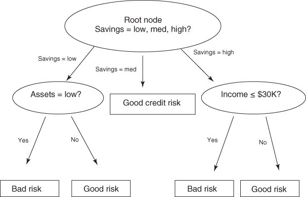
Figure 11.1 Simple decision tree.
The target variable for the decision tree in Figure 11.1 is credit risk, with potential customers being classified as either good or bad credit risks. The predictor variables are savings (low, medium, and high), assets (low or not low), and income (≤$30,000 or >$30,000). Here, the root node represents a decision node, testing whether each record has a low, medium, or high savings level (as defined by the analyst or domain expert). The data set is partitioned, or split, according to the values of this attribute. Those records with low savings are sent via the leftmost branch (savings = low) to another decision node. The records with high savings are sent via the rightmost branch to a different decision node.
The records with medium savings are sent via the middle branch directly to a leaf node, indicating the termination of this branch. Why a leaf node and not another decision node? Because, in the data set (not shown), all of the records with medium savings levels have been classified as good credit risks. There is no need for another decision node, because our knowledge that the customer has medium savings predicts good credit with 100% accuracy in the data set.
For customers with low savings, the next decision node tests whether the customer has low assets. Those with low assets are then classified as bad credit risks; the others are classified as good credit risks. For customers with high savings, the next decision node tests whether the customer has an income of at most $30,000. Customers with incomes of $30,000 or less are then classified as bad credit risks, with the others classified as good credit risks.
When no further splits can be made, the decision tree algorithm stops growing new nodes. For example, suppose that all of the branches terminate in “pure” leaf nodes, where the target variable is unary for the records in that node (e.g., each record in the leaf node is a good credit risk). Then no further splits are necessary, so no further nodes are grown.
However, there are instances when a particular node contains “diverse” attributes (with non-unary values for the target attribute), and yet the decision tree cannot make a split. For example, suppose that we consider the records from Figure 11.1 with high savings and low income (≤$30,000). Suppose that there are five records with these values, all of which also have low assets. Finally, suppose that three of these five customers have been classified as bad credit risks and two as good credit risks, as shown in Table 11.1. In the real world, one often encounters situations such as this, with varied values for the response variable, even for exactly the same values for the predictor variables.
Table 11.1 Sample of records that cannot lead to pure leaf node
| Customer | Savings | Assets | Income | Credit Risk |
| 004 | High | Low | ≤$30,000 | Good |
| 009 | High | Low | ≤$30,000 | Good |
| 027 | High | Low | ≤$30,000 | Bad |
| 031 | High | Low | ≤$30,000 | Bad |
| 104 | High | Low | ≤$30,000 | Bad |
Here, as all customers have the same predictor values, there is no possible way to split the records according to the predictor variables that will lead to a pure leaf node. Therefore, such nodes become diverse leaf nodes, with mixed values for the target attribute. In this case, the decision tree may report that the classification for such customers is “bad,” with 60% confidence, as determined by the three-fifths of customers in this node who are bad credit risks. Note that not all attributes are tested for all records. Customers with low savings and low assets, for example, are not tested with regard to income in this example.
11.2 Requirements for Using Decision Trees
Following requirements must be met before decision tree algorithms may be applied:
- Decision tree algorithms represent supervised learning, and as such require preclassified target variables. A training data set must be supplied, which provides the algorithm with the values of the target variable.
- This training data set should be rich and varied, providing the algorithm with a healthy cross section of the types of records for which classification may be needed in the future. Decision trees learn by example, and if examples are systematically lacking for a definable subset of records, classification and prediction for this subset will be problematic or impossible.
- The target attribute classes must be discrete. That is, one cannot apply decision tree analysis to a continuous target variable. Rather, the target variable must take on values that are clearly demarcated as either belonging to a particular class or not belonging.
Why, in the example above, did the decision tree choose the savings attribute for the root node split? Why did it not choose assets or income instead? Decision trees seek to create a set of leaf nodes that are as “pure” as possible; that is, where each of the records in a particular leaf node has the same classification. In this way, the decision tree may provide classification assignments with the highest measure of confidence available.
However, how does one measure uniformity, or conversely, how does one measure heterogeneity? We shall examine two of the many methods for measuring leaf node purity, which lead to the following two leading algorithms for constructing decision trees:
- Classification and regression trees (CART) algorithm;
- C4.5 algorithm.
11.3 Classification and Regression Trees
The CART method was suggested by Breiman et al.1 in 1984. The decision trees produced by CART are strictly binary, containing exactly two branches for each decision node. CART recursively partitions the records in the training data set into subsets of records with similar values for the target attribute. The CART algorithm grows the tree by conducting for each decision node, an exhaustive search of all available variables and all possible splitting values, selecting the optimal split according to the following criteria (from Kennedy et al.2).
Let Φ(s|t) be a measure of the “goodness” of a candidate split s at node t, where

and where

Then the optimal split is whichever split maximizes this measure Φ(s|t) over all possible splits at node t.
Let us look at an example. Suppose that we have the training data set shown in Table 11.2 and are interested in using CART to build a decision tree for predicting whether a particular customer should be classified as being a good or a bad credit risk. In this small example, all eight training records enter into the root node. As CART is restricted to binary splits, the candidate splits that the CART algorithm would evaluate for the initial partition at the root node are shown in Table 11.3. Although income is a continuous variable, CART may still identify a finite list of possible splits based on the number of different values that the variable actually takes in the data set. Alternatively, the analyst may choose to categorize the continuous variable into a smaller number of classes.
Table 11.2 Training set of records for classifying credit risk
| Customer | Savings | Assets | Income ($1000s) | Credit Risk |
| 1 | Medium | High | 75 | Good |
| 2 | Low | Low | 50 | Bad |
| 3 | High | Medium | 25 | Bad |
| 4 | Medium | Medium | 50 | Good |
| 5 | Low | Medium | 100 | Good |
| 6 | High | High | 25 | Good |
| 7 | Low | Low | 25 | Bad |
| 8 | Medium | Medium | 75 | Good |
Table 11.3 Candidate splits for t = root node
| Candidate Split | Left Child Node, tL | Right Child Node, tR |
| 1 | Savings = low | Savings ∈ {medium, high} |
| 2 | Savings = medium | Savings ∈ {low, high} |
| 3 | Savings = high | Savings ∈ {low, medium} |
| 4 | Assets = low | Assets ∈ {medium, high} |
| 5 | Assets = medium | Assets ∈ {low, high} |
| 6 | Assets = high | Assets ∈ {low, medium} |
| 7 | Income ≤ $25,000 | Income > $25,000 |
| 8 | Income ≤ $50,000 | Income > $50,000 |
| 9 | Income ≤ $75,000 | Income > $75,000 |
For each candidate split, let us examine the values of the various components of the optimality measure Φ(s|t) in Table 11.4. Using these observed values, we may investigate the behavior of the optimality measure under various conditions. For example, when is Φ(s|t) large? We see that Φ(s|t) is large when both of its main components are large: 2PLPR and ![]() .
.
Table 11.4 Values of the components of the optimality measure Φ(s|t) for each candidate split, for the root node (best performance highlighted)
| Split | PL | PR | P(j|tL) | P(j|tR) | 2PLPR | Q(s|t) | Φ(s|t) |
| 1 | 0.375 | 0.625 | G: 0.333 | G: 0.8 | 0.46875 | 0.934 | 0.4378 |
| B: 0.667 | B: 0.2 | ||||||
| 2 | 0.375 | 0.625 | G: 1 | G: 0.4 | 0.46875 | 1.2 | 0.5625 |
| B: 0 | B: 0.6 | ||||||
| 3 | 0.25 | 0.75 | G: 0.5 | G: 0.667 | 0.375 | 0.334 | 0.1253 |
| B: 0.5 | B: 0.333 | ||||||
| 4 | 0.25 | 0.75 | G: 0 | G: 0.833 | 0.375 | 1.667 | 0.6248 |
| B: 1 | B: 0.167 | ||||||
| 5 | 0.5 | 0.5 | G: 0.75 | G: 0.5 | 0.5 | 0.5 | 0.25 |
| B: 0.25 | B: 0.5 | ||||||
| 6 | 0.25 | 0.75 | G: 1 | G: 0.5 | 0.375 | 1 | 0.375 |
| B: 0 | B: 0.5 | ||||||
| 7 | 0.375 | 0.625 | G: 0.333 | G: 0.8 | 0.46875 | 0.934 | 0.4378 |
| B: 0.667 | B: 0.2 | ||||||
| 8 | 0.625 | 0.375 | G: 0.4 | G: 1 | 0.46875 | 1.2 | 0.5625 |
| B: 0.6 | B: 0 | ||||||
| 9 | 0.875 | 0.125 | G: 0.571 | G: 1 | 0.21875 | 0.858 | 0.1877 |
| B: 0.429 | B: 0 |
Consider ![]() . When is the component Q(s|t) large? Q(s|t) is large when the distance between P(j|tL) and P(j|tR) is maximized across each class (value of the target variable). In other words, this component is maximized when the proportions of records in the child nodes for each particular value of the target variable are as different as possible. The maximum value would therefore occur when for each class the child nodes are completely uniform (pure). The theoretical maximum value for Q(s|t) is k, where k is the number of classes for the target variable. As our output variable credit risk takes two values, good and bad, k = 2 is the maximum for this component.
. When is the component Q(s|t) large? Q(s|t) is large when the distance between P(j|tL) and P(j|tR) is maximized across each class (value of the target variable). In other words, this component is maximized when the proportions of records in the child nodes for each particular value of the target variable are as different as possible. The maximum value would therefore occur when for each class the child nodes are completely uniform (pure). The theoretical maximum value for Q(s|t) is k, where k is the number of classes for the target variable. As our output variable credit risk takes two values, good and bad, k = 2 is the maximum for this component.
The component 2PLPR is maximized when PL and PR are large, which occurs when the proportions of records in the left and right child nodes are equal. Therefore, Φ(s|t) will tend to favor balanced splits that partition the data into child nodes containing roughly equal numbers of records. Hence, the optimality measure Φ(s|t) prefers splits that will provide child nodes that are homogeneous for all classes and have roughly equal numbers of records. The theoretical maximum for 2PLPR is 2(0.5)(0.5) = 0.5.
In this example, only candidate split 5 has an observed value for 2PLPR that reaches the theoretical maximum for this statistic, 0.5, because the records are partitioned equally into two groups of four. The theoretical maximum for Q(s|t) is obtained only when each resulting child node is pure, and thus is not achieved for this data set.
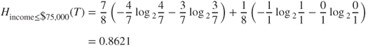
The maximum observed value for Φ(s|t) among the candidate splits is therefore attained by split 4, with Φ(s|t) = 0.6248. CART therefore chooses to make the initial partition of the data set using candidate split 4, assets = low versus assets ∈{medium, high}, as shown in Figure 11.2.

Figure 11.2 CART decision tree after initial split.
The left child node turns out to be a terminal leaf node, because both of the records that were passed to this node had bad credit risk. The right child node, however, is diverse and calls for further partitioning.
We again compile a table of the candidate splits (all are available except split 4), along with the values for the optimality measure (Table 11.5). Here two candidate splits (3 and 7) share the highest value for Φ(s|t), 0.4444. We arbitrarily select the first split encountered, split 3, savings = high versus savings ∈{low, medium}, for decision node A, with the resulting tree shown in Figure 11.3.
Table 11.5 Values of the components of the optimality measure Φ(s|t) for each candidate split, for decision node A (best performance highlighted)
| Split | PL | PR | P(j|tL) | P(j|tR) | 2PLPR | Q(s|t) | Φ(s|t) |
| 1 | 0.167 | 0.833 | G: 1 | G: 0.8 | 0.2782 | 0.4 | 0.1113 |
| B: 0 | B: 0.2 | ||||||
| 2 | 0.5 | 0.5 | G: 1 | G: 0.667 | 0.5 | 0.6666 | 0.3333 |
| B: 0 | B: 0.333 | ||||||
| 3 | 0.333 | 0.667 | G: 0.5 | G: 1 | 0.4444 | 1 | 0.4444 |
| B: 0.5 | B: 0 | ||||||
| 5 | 0.667 | 0.333 | G: 0.75 | G: 1 | 0.4444 | 0.5 | 0.2222 |
| B: 0.25 | B: 0 | ||||||
| 6 | 0.333 | 0.667 | G: 1 | G: 0.75 | 0.4444 | 0.5 | 0.2222 |
| B: 0 | B: 0.25 | ||||||
| 7 | 0.333 | 0.667 | G: 0.5 | G: 1 | 0.4444 | 1 | 0.4444 |
| B: 0.5 | B: 0 | ||||||
| 8 | 0.5 | 0.5 | G: 0.667 | G: 1 | 0.5 | 0.6666 | 0.3333 |
| B: 0.333 | B: 0 | ||||||
| 9 | 0.833 | 0.167 | G: 0.8 | G: 1 | 0.2782 | 0.4 | 0.1113 |
| B: 0.2 | B: 0 |

Figure 11.3 CART decision tree after decision node A split.
As decision node B is diverse, we again need to seek the optimal split. Only two records remain in this decision node, each with the same value for savings (high) and income (25). Therefore, the only possible split is assets = high versus assets = medium, providing us with the final form of the CART decision tree for this example, in Figure 11.4. Compare Figure 11.4 with Figure 11.5, the decision tree generated by Modeler's CART algorithm.

Figure 11.4 CART decision tree, fully grown form.

Figure 11.5 Modeler's CART decision tree.
Let us leave aside this example now, and consider how CART would operate on an arbitrary data set. In general, CART would recursively proceed to visit each remaining decision node and apply the procedure above to find the optimal split at each node. Eventually, no decision nodes remain, and the “full tree” has been grown. However, as we have seen in Table 11.1, not all leaf nodes are necessarily homogeneous, which leads to a certain level of classification error.
For example, suppose that, as we cannot further partition the records in Table 11.1, we classify the records contained in this leaf node as bad credit risk. Then the probability that a randomly chosen record from this leaf node would be classified correctly is 0.6, because three of the five records (60%) are actually classified as bad credit risks. Hence, our classification error rate for this particular leaf would be 0.4 or 40%, because two of the five records are actually classified as good credit risks. CART would then calculate the error rate for the entire decision tree to be the weighted average of the individual leaf error rates, with the weights equal to the proportion of records in each leaf.
To avoid memorizing the training set, the CART algorithm needs to begin pruning nodes and branches that would otherwise reduce the generalizability of the classification results. Even though the fully grown tree has the lowest error rate on the training set, the resulting model may be too complex, resulting in overfitting. As each decision node is grown, the subset of records available for analysis becomes smaller and less representative of the overall population. Pruning the tree will increase the generalizability of the results. How the CART algorithm performs tree pruning is explained in Breiman et al. [p. 66]. Essentially, an adjusted overall error rate is found that penalizes the decision tree for having too many leaf nodes and thus too much complexity.
11.4 C4.5 Algorithm
The C4.5 algorithm is Quinlan's extension of his own iterative dichotomizer 3 (ID3) algorithm for generating decision trees.3 Just as with CART, the C4.5 algorithm recursively visits each decision node, selecting the optimal split, until no further splits are possible. However, there are following interesting differences between CART and C4.5:
- Unlike CART, the C4.5 algorithm is not restricted to binary splits. Whereas CART always produces a binary tree, C4.5 produces a tree of more variable shape.
- For categorical attributes, C4.5 by default produces a separate branch for each value of the categorical attribute. This may result in more “bushiness” than desired, because some values may have low frequency or may naturally be associated with other values.
- The C4.5 method for measuring node homogeneity is quite different from the CART method and is examined in detail below.
The C4.5 algorithm uses the concept of information gain or entropy reduction to select the optimal split. Suppose that we have a variable X whose k possible values have probabilities p1, p2, …, pk. What is the smallest number of bits, on average per symbol, needed to transmit a stream of symbols representing the values of X observed? The answer is called the entropy of X and is defined as
Where does this formula for entropy come from? For an event with probability p, the average amount of information in bits required to transmit the result is −log2(p). For example, the result of a fair coin toss, with probability 0.5, can be transmitted using −log2(0.5) = 1 bit, which is a 0 or 1, depending on the result of the toss. For variables with several outcomes, we simply use a weighted sum of the log2(pj)s, with weights equal to the outcome probabilities, resulting in the formula
C4.5 uses this concept of entropy as follows. Suppose that we have a candidate split S, which partitions the training data set T into several subsets, T1, T2, …, Tk. The mean information requirement can then be calculated as the weighted sum of the entropies for the individual subsets, as follows:

where Pi represents the proportion of records in subset i. We may then define our information gain to be gain(S) = H(T) − HS(T), that is, the increase in information produced by partitioning the training data T according to this candidate split S. At each decision node, C4.5 chooses the optimal split to be the split that has the greatest information gain, gain(S).
To illustrate the C4.5 algorithm at work, let us return to the data set in Table 11.2 and apply the C4.5 algorithm to build a decision tree for classifying credit risk, just as we did earlier using CART. Once again, we are at the root node and are considering all possible splits using all the data (Table 11.6).
Table 11.6 Candidate splits at root node for C4.5 algorithm
| Candidate Split | Child Nodes | ||
| 1 | Savings = low | Savings = medium | Savings = high |
| 2 | Assets = low | Assets = medium | Assets = high |
| 3 | Income ≤ $25,000 | Income > $25,000 | |
| 4 | Income ≤ $50,000 | Income > $50,000 | |
| 5 | Income ≤ $75,000 | Income > $75,000 |
Now, because five of the eight records are classified as good credit risk, with the remaining three records classified as bad credit risk, the entropy before splitting is
We shall compare the entropy of each candidate split against this H(T) = 0.9544, to see which split results in the greatest reduction in entropy (or gain in information).
For candidate split 1 (savings), two of the records have high savings, three of the records have medium savings, and three of the records have low savings, so we have ![]() . Of the records with high savings, one is a good credit risk and one is bad, giving a probability of 0.5 of choosing the record with a good credit risk. Thus, the entropy for high savings is
. Of the records with high savings, one is a good credit risk and one is bad, giving a probability of 0.5 of choosing the record with a good credit risk. Thus, the entropy for high savings is ![]() , which is similar to the flip of a fair coin. All three of the records with medium savings are good credit risks, so that the entropy for medium is
, which is similar to the flip of a fair coin. All three of the records with medium savings are good credit risks, so that the entropy for medium is ![]() , where by convention we define log2(0) = 0.
, where by convention we define log2(0) = 0.
In engineering applications, information is analogous to signal, and entropy is analogous to noise, so it makes sense that the entropy for medium savings is zero, because the signal is crystal clear and there is no noise: If the customer has medium savings, he or she is a good credit risk, with 100% confidence. The amount of information required to transmit the credit rating of these customers is zero, as long as we know that they have medium savings.
One of the records with low savings is a good credit risk, and two records with low savings are bad credit risks, giving us our entropy for low credit risk as ![]() . We combine the entropies of these three subsets, using equation (11.2) and the proportions of the subsets Pi, so that
. We combine the entropies of these three subsets, using equation (11.2) and the proportions of the subsets Pi, so that ![]() . Then the information gain represented by the split on the savings attribute is calculated as H(T) − Hsavings(T) = 0.9544 − 0.5944 = 0.36 bits.
. Then the information gain represented by the split on the savings attribute is calculated as H(T) − Hsavings(T) = 0.9544 − 0.5944 = 0.36 bits.
How are we to interpret these measures? First, H(T) = 0.9544 means that, on average, one would need 0.9544 bits (0's or 1's) to transmit the credit risk of the eight customers in the data set. Now, Hsavings(T) = 0.5944 means that the partitioning of the customers into three subsets has lowered the average bit requirement for transmitting the credit risk status of the customers to 0.5944 bits. Lower entropy is good. This entropy reduction can be viewed as information gain, so that we have gained on average H(T) − Hsavings(T) = 0.9544 − 0.5944 = 0.36 bits of information by using the savings partition. We will compare this to the information gained by the other candidate splits, and choose the split with the largest information gain as the optimal split for the root node.
For candidate split 2 (assets), two of the records have high assets, four of the records have medium assets, and two of the records have low assets, so we have ![]() . Both of the records with high assets are classified as good credit risks, which means that the entropy for high assets will be zero, just as it was for medium savings above.
. Both of the records with high assets are classified as good credit risks, which means that the entropy for high assets will be zero, just as it was for medium savings above.
Three of the records with medium assets are good credit risks and one is a bad credit risk, giving us entropy ![]() . And both of the records with low assets are bad credit risks, which results in the entropy for low assets equaling zero. Combining the entropies of these three subsets, using equation (11.2) and the proportions of the subsets Pi, we have
. And both of the records with low assets are bad credit risks, which results in the entropy for low assets equaling zero. Combining the entropies of these three subsets, using equation (11.2) and the proportions of the subsets Pi, we have ![]() . The entropy for the assets split is lower than the entropy (0.5944) for the savings split, which indicates that the assets split contains less noise and is to be preferred over the savings split. This is measured directly using the information gain, as follows: H(T) − Hassets(T) = 0.9544 − 0.4057 = 0.5487 bits. This information gain of 0.5487 bits is larger than that for the savings split of 0.36 bits, verifying that the assets split is preferable.
. The entropy for the assets split is lower than the entropy (0.5944) for the savings split, which indicates that the assets split contains less noise and is to be preferred over the savings split. This is measured directly using the information gain, as follows: H(T) − Hassets(T) = 0.9544 − 0.4057 = 0.5487 bits. This information gain of 0.5487 bits is larger than that for the savings split of 0.36 bits, verifying that the assets split is preferable.
While C4.5 partitions the categorical variables differently from CART, the partitions for the numerical variables are similar. Here we have four observed values for income: 25,000, 50,000, 75,000, and 100,000, which provide us with three thresholds for partitions, as shown in Table 11.6. For candidate split 3 from Table 11.6, income ≤ $25,000 versus income > $25,000, three of the records have income ≤ $25,000, with the other five records having income > $25,000, giving us ![]() . Of the records with income ≤ $25,000, one is a good credit risk and two are bad, giving us the entropy for income ≤ $25,000 as
. Of the records with income ≤ $25,000, one is a good credit risk and two are bad, giving us the entropy for income ≤ $25,000 as ![]() . Four of the five records with income > $25,000 are good credit risks, so that the entropy for income > $25,000 is
. Four of the five records with income > $25,000 are good credit risks, so that the entropy for income > $25,000 is ![]() . Combining, we find the entropy for candidate split 3 to be
. Combining, we find the entropy for candidate split 3 to be ![]() . Then the information gain for this split is
. Then the information gain for this split is ![]() bits, which is our poorest choice yet.
bits, which is our poorest choice yet.
For candidate split 4, income ≤ $50,000 versus income > $50,000, two of the five records with income ≤ $50,000 are good credit risks, and three are bad, while all three of the records with income > $50,000 are good credit risks. This gives us the entropy for candidate split 4 as

The information gain for this split is thus H(T) − Hincome ≤ $50,000(T) = 0.9544 − 0.6069 = 0.3475, which is not as good as for assets. Finally, for candidate split 5, income ≤ $75,000 versus income > $75,000, four of the seven records with income ≤ $75,000 are good credit risks, and three are bad, while the single record with income > $75,000 is a good credit risk. Thus, the entropy for candidate split 4 is
The information gain for this split is H(T) − Hincome ≤ $75,000(T) = 0.9544 − 0.8621 = 0.0923, making this split the poorest of the five candidate splits.
Table 11.7 summarizes the information gain for each candidate split at the root node. Candidate split 2, assets, has the largest information gain, and so is chosen for the initial split by the C4.5 algorithm. Note that this choice for an optimal split concurs with the partition preferred by CART, which split on assets = low versus assets = {medium, high}. The partial decision tree resulting from C4.5's initial split is shown in Figure 11.6.
Table 11.7 Information gain for each candidate split at the root node
| Candidate Split | Child Nodes | Information Gain (Entropy Reduction) |
| 1 | Savings = low | 0.36 bits |
| Savings = medium | ||
| Savings = high | ||
| 2 | Assets = low | 0.5487 bits |
| Assets = medium | ||
| Assets = high | ||
| 3 | Income ≤ $25,000 | 0.1588 bits |
| Income > $25,000 | ||
| 4 | Income ≤ $50,000 | 0.3475 bits |
| Income > $50,000 | ||
| 5 | Income ≤ $75,000 | 0.0923 bits |
| Income > $75,000 |
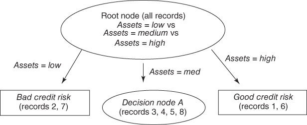
Figure 11.6 C4.5 concurs with CART in choosing assets for the initial partition.
The initial split has resulted in the creation of two terminal leaf nodes and one new decision node. As both records with low assets have bad credit risk, this classification has 100% confidence, and no further splits are required. It is similar for the two records with high assets. However, the four records at decision node A (assets = medium) contain both good and bad credit risks, so that further splitting is called for.
We proceed to determine the optimal split for decision node A, containing records 3, 4, 5, and 8, as indicated in Table 11.8. Because three of the four records are classified as good credit risks, with the remaining record classified as a bad credit risk, the entropy before splitting is
Table 11.8 Records available at decision node A for classifying credit risk
| Customer | Savings | Assets | Income ($1000s) | Credit Risk |
| 3 | High | Medium | 25 | Bad |
| 4 | Medium | Medium | 50 | Good |
| 5 | Low | Medium | 100 | Good |
| 8 | Medium | Medium | 75 | Good |
The candidate splits for decision node A are shown in Table 11.9.
Table 11.9 Candidate splits at decision node A
| Candidate Split | Child Nodes | ||
| 1 | Savings = low | Savings = medium | Savings = high |
| 3 | Income ≤ $25,000 | Income > $25,000 | |
| 4 | Income ≤ $50,000 | Income > $50,000 | |
| 5 | Income ≤ $75,000 | Income > $75,000 |
For candidate split 1, savings, the single record with low savings is a good credit risk, along with the two records with medium savings. Perhaps counterintuitively, the single record with high savings is a bad credit risk. So the entropy for each of these three classes equals zero, because the level of savings determines the credit risk completely. This also results in a combined entropy of zero for the assets split, Hassets(A) = 0, which is optimal for decision node A. The information gain for this split is thus H(A) − Hassets(A) = 0.8113 − 0.0 = 0.8113. This is, of course, the maximum information gain possible for decision node A. We therefore need not continue our calculations, because no other split can result in a greater information gain. As it happens, candidate split 3, income ≤ $25,000 versus income > $25,000, also results in the maximal information gain, but again we arbitrarily select the first such split encountered, the savings split.
Figure 11.7 shows the form of the decision tree after the savings split. Note that this is the fully grown form, because all nodes are now leaf nodes, and C4.5 will grow no further nodes. Comparing the C4.5 tree in Figure 11.7 with the CART tree in Figure 11.4, we see that the C4.5 tree is “bushier,” providing a greater breadth, while the CART tree is one level deeper. Both algorithms concur that assets is the most important variable (the root split) and that savings is also important. Finally, once the decision tree is fully grown, C4.5 engages in pessimistic postpruning. Interested readers may consult Kantardzic.4
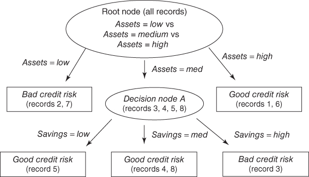
Figure 11.7 C4.5 Decision tree: fully grown form.
11.5 Decision Rules
One of the most attractive aspects of decision trees lies in their interpretability, especially with respect to the construction of decision rules. Decision rules can be constructed from a decision tree simply by traversing any given path from the root node to any leaf. The complete set of decision rules generated by a decision tree is equivalent (for classification purposes) to the decision tree itself. For example, from the decision tree in Figure 11.7, we may construct the decision rules given in Table 11.10.
Table 11.10 Decision rules generated from decision tree in Figure 11.7
| Antecedent | Consequent | Support | Confidence |
| If assets = low | then bad credit risk | 1.00 | |
| If assets = high | then good credit risk | 1.00 | |
| If assets = medium and savings = low | then good credit risk | 1.00 | |
| If assets = medium and savings = medium | then good credit risk | 1.00 | |
| If assets = medium and savings = high | then bad credit risk | 1.00 |
Decision rules come in the form if antecedent, then consequent, as shown in Table 11.10. For decision rules, the antecedent consists of the attribute values from the branches taken by the particular path through the tree, while the consequent consists of the classification value for the target variable given by the particular leaf node.
The support of the decision rule refers to the proportion of records in the data set that rest in that particular terminal leaf node. The confidence of the rule refers to the proportion of records in the leaf node for which the decision rule is true. In this small example, all of our leaf nodes are pure, resulting in perfect confidence levels of 100% = 1.00. In real-world examples, such as in the next section, one cannot expect such high confidence levels.
11.6 Comparison of the C5.0 and CART Algorithms Applied to Real Data
Next, we apply decision tree analysis using IBM/SPSS Modeler on a real-world data set. We use a subset of the data set adult, which was drawn from US census data by Kohavi.5 You may download the data set used here from the book series website, www.dataminingconsultant.com. Here we are interested in classifying whether or not a person's income is less than $50,000, based on the following set of predictor fields.
- Numerical variables
- Age
- Years of education
- Capital gains
- Capital losses
- Hours worked per week.
- Categorical variables
- Race
- Gender
- Work class
- Marital status.
The numerical variables were normalized so that all values ranged between 0 and 1. Some collapsing of low-frequency classes was carried out on the work class and marital status categories. Modeler was used to compare the C5.0 algorithm (an update of the C4.5 algorithm) with CART. The decision tree produced by the CART algorithm is shown in Figure 11.8.
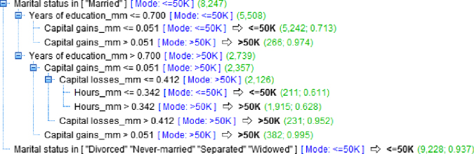
Figure 11.8 CART decision tree for the adult data set.
Here, the tree structure is displayed horizontally, with the root node at the left and the leaf nodes on the right. For the CART algorithm, the root node split is on marital status, with a binary split separating married persons from all others (Marital_Status in [“Divorced” “Never-married” “Separated” “Widowed”]). That is, this particular split on marital status maximized the CART split selection criterion [equation (11.1)]:

Note that the mode classification for each branch is less than or equal to $50,000. The married branch leads to a decision node, with several further splits downstream. However, the nonmarried branch is a leaf node, with a classification of less than or equal to $50,000 for the 9228 such records, with 93.7% confidence. In other words, of the 9228 persons in the data set who are not presently married, 93.7% of them have incomes of at most $50,000.
The root node split is considered to indicate the most important single variable for classifying income. Note that the split on the Marital_Status attribute is binary, as are all CART splits on categorical variables. All the other splits in the full CART decision tree shown in Figure 11.8 are on numerical variables. The next decision node is Years of education_mm, representing the min–max normalized number of years of education. The split occurs at Years of education_mm ![]() (mode ≤ $50,000) versus Years of education_mm
(mode ≤ $50,000) versus Years of education_mm ![]() (mode > $50,000). However, your client may not understand what the normalized value of 0.700 represents. So, when reporting results, the analyst should always denormalize, to identify the original field values. The min–max normalization was of the form
(mode > $50,000). However, your client may not understand what the normalized value of 0.700 represents. So, when reporting results, the analyst should always denormalize, to identify the original field values. The min–max normalization was of the form ![]() . Years of education ranged from 16 (maximum) to 1 (minimum), for a range of 15. Therefore, denormalizing, we have
. Years of education ranged from 16 (maximum) to 1 (minimum), for a range of 15. Therefore, denormalizing, we have ![]()
. Thus, the split occurs at 11.5 years of education. It seems that those who have graduated high school tend to have higher incomes than those who have not.
Interestingly, for both education groups, Capital gains represents the next most important decision node. For the branch with more years of education, there are two further splits, on Capital loss, and then Hours (worked per week).
Now, will the information-gain splitting criterion and the other characteristics of the C5.0 algorithm lead to a decision tree that is substantially different from or largely similar to the tree derived using CART's splitting criteria? Compare the CART decision tree above with Modeler's C5.0 decision tree of the same data displayed in Figure 11.9. (We needed to specify only three levels of splits. Modeler gave us eight levels of splits, which would not have fit on the page.)

Figure 11.9 C5.0 decision tree for the adult data set.
Differences emerge immediately at the root node. Here, the root split is on the Capital gains_mm attribute, with the split occurring at the relatively low normalized level of 0.068. As the range of capital gains in this data set is $99,999 (maximum = 99,999, minimum = 0), this is denormalized as ![]() . More than half of those with capital gains greater than $6850 have incomes above $50,000, whereas more than half of those with capital gains of less than $6850 have incomes below $50,000. This is the split that was chosen by the information-gain criterion as the optimal split among all possible splits over all fields. Note, however, that there are 23 times more records in the low-capital-gains category than in the high-capital-gains category (23,935 vs 1065 records).
. More than half of those with capital gains greater than $6850 have incomes above $50,000, whereas more than half of those with capital gains of less than $6850 have incomes below $50,000. This is the split that was chosen by the information-gain criterion as the optimal split among all possible splits over all fields. Note, however, that there are 23 times more records in the low-capital-gains category than in the high-capital-gains category (23,935 vs 1065 records).
For records with lower capital gains, the second split occurs on capital loss, with a pattern similar to the earlier split on capital gains. Most people (23,179 records) had low capital loss, and most of these have incomes below $50,000. Most of the few (756 records) who had higher capital loss had incomes above $50,000.
For records with low capital gains and low capital loss, consider the next split, which is made on marital status. Note that C5.0 provides a separate branch for each categorical field value, whereas CART was restricted to binary splits. A possible drawback of C5.0's strategy for splitting categorical variables is that it may lead to an overly bushy tree, with many leaf nodes containing few records.
Although the CART and C5.0 decision trees do not agree in the details, we may nevertheless glean useful information from the broad areas of agreement between them. For example, the most important variables are clearly marital status, education, capital gains, capital losses, and perhaps hours per week. Both models agree that these fields are important, but disagree as to the ordering of their importance. Much more modeling analysis may be called for.
For a soup-to-nuts application of decision trees to a real-world data set, from data preparation through model building and decision rule generation, see the Case Study in Chapter 29–32.
R References
- 1 Kuhn M, Weston S, Coulter N. 2013. C code for C5.0 by R. Quinlan. C50: C5.0 decision trees and rule-based models. R package version 0.1.0-15. http://CRAN.R-project.org/package=C50.
- 2 Milborrow S. 2012. rpart.plot: Plot rpart models. An enhanced version of plot.rpart. R package version 1.4-3. http://CRAN.R-project.org/package=rpart.plot.
- 3 Therneau T, Atkinson B, Ripley B. 2013. rpart: Recursive partitioning. R package version 4.1-3. http://CRAN.R-project.org/package=rpart.
- 4 R Core Team. R: A Language and Environment for Statistical Computing. Vienna, Austria: R Foundation for Statistical Computing; 2012. ISBN: 3-900051-07-0, http://www.R-project.org/.
Exercises
Clarifying The Concepts
1. Describe the possible situations when no further splits can be made at a decision node.
2. Suppose that our target variable is continuous numeric. Can we apply decision trees directly to classify it? How can we work around this?
3. True or false: Decision trees seek to form leaf nodes to maximize heterogeneity in each node.
4. Discuss the benefits and drawbacks of a binary tree versus a bushier tree.
Working With The Data
Consider the data in Table 11.11. The target variable is salary. Start by discretizing salary as follows:
- • Less than $35,000, Level 1
- • $35,000 to less than $45,000, Level 2
- • $45,000 to less than $55,000, Level 3
- • Above $55,000, Level 4.
Table 11.11 Decision tree data
| Occupation | Gender | Age | Salary |
| Service | Female | 45 | $48,000 |
| Male | 25 | $25,000 | |
| Male | 33 | $35,000 | |
| Management | Male | 25 | $45,000 |
| Female | 35 | $65,000 | |
| Male | 26 | $45,000 | |
| Female | 45 | $70,000 | |
| Sales | Female | 40 | $50,000 |
| Male | 30 | $40,000 | |
| Staff | Female | 50 | $40,000 |
| Male | 25 | $25,000 |
5. Construct a classification and regression tree to classify salary based on the other variables. Do as much as you can by hand, before turning to the software.
6. Construct a C4.5 decision tree to classify salary based on the other variables. Do as much as you can by hand, before turning to the software.
7. Compare the two decision trees and discuss the benefits and drawbacks of each.
8. Generate the full set of decision rules for the CART decision tree.
9. Generate the full set of decision rules for the C4.5 decision tree.
10. Compare the two sets of decision rules and discuss the benefits and drawbacks of each.
Hands-On Analysis
For the following exercises, use the churn data set available at the book series web site. Normalize the numerical data and deal with the correlated variables.
11. Generate a CART decision tree.
12. Generate a C4.5-type decision tree.
13. Compare the two decision trees and discuss the benefits and drawbacks of each.
14. Generate the full set of decision rules for the CART decision tree.
15. Generate the full set of decision rules for the C4.5 decision tree.
16. Compare the two sets of decision rules and discuss the benefits and drawbacks of each.