
Chapter 12
Neural Networks
The inspiration for neural networks was the recognition that complex learning systems in the animal brains consisted of closely interconnected sets of neurons. Although a particular neuron may be relatively simple in structure, dense networks of interconnected neurons could perform complex learning tasks such as classification and pattern recognition. The human brain, for example, contains approximately 1011 neurons, each connected on average to 10,000 other neurons, making a total of 1,000,000,000,000,000 = 1015 synaptic connections. Artificial neural networks (hereafter, neural networks) represent an attempt at a very basic level to imitate the type of nonlinear learning that occurs in the networks of neurons found in nature.
As shown in Figure 12.1, a real neuron uses dendrites to gather inputs from other neurons and combines the input information, generating a nonlinear response (“firing”) when some threshold is reached, which it sends to other neurons using the axon. Figure 12.1 also shows an artificial neuron model used in most neural networks. The inputs (xi) are collected from upstream neurons (or the data set) and combined through a combination function such as summation (∑), which is then input into (usually nonlinear) activation function to produce an output response (y), which is then channeled downstream to other neurons.

Figure 12.1 Real neuron and artificial neuron model.
What types of problems are appropriate for neural networks? One of the advantages of using neural networks is that they are quite robust with respect to noisy data. Because the network contains many nodes (artificial neurons), with weights assigned to each connection, the network can learn to work around these uninformative (or even erroneous) examples in the data set. However, unlike decision trees, which produce intuitive rules that are understandable to nonspecialists, neural networks are relatively opaque to human interpretation, as we shall see. Also, neural networks usually require longer training times than decision trees, often extending into several hours.
12.1 Input and Output Encoding
One possible drawback of neural networks is that all attribute values must be encoded in a standardized manner, taking values between 0 and 1, even for categorical variables. Later, when we examine the details of the back-propagation algorithm, we shall understand why this is necessary. For now, however, how does one go about standardizing all the attribute values?
For continuous variables, this is not a problem, as we discussed in Chapter 2. We may simply apply the min–max normalization:
This works well as long as the minimum and maximum values are known and all potential new data are bounded between them. Neural networks are somewhat robust to minor violations of these boundaries. If more serious violations are expected, certain ad hoc solutions may be adopted, such as rejecting values that are outside the boundaries, or assigning such values to either the minimum or the maximum value.
Categorical variables are more problematical, as might be expected. If the number of possible categories is not too large, one may use indicator (flag) variables. For example, many data sets contain a gender attribute, containing values female, male, and unknown. As the neural network could not handle these attribute values in their present form, we could, instead, create indicator variables for female and male. Each record would contain values for each of these two indicator variables. Records for females would have values of 1 for female and 0 for male, while records for males would have values of 0 for female and 1 for male. Records for persons of unknown gender would have values of 0 for female and 0 for male. In general, categorical variables with k classes may be translated into k − 1 indicator variables, as long as the definition of the indicators is clearly defined.
Be wary of recoding unordered categorical variables into a single variable with a range between 0 and 1. For example, suppose that the data set contains information on a marital status attribute. Suppose that we code the attribute values divorced, married, separated, single, widowed, and unknown, as 0.0, 0.2, 0.4, 0.6, 0.8, and 1.0, respectively. Then this coding implies, for example, that divorced is “closer” to married than it is to separated, and so on. The neural network would be aware only of the numerical values in the marital status field, not of their preencoded meanings, and would thus be naive of their true meaning. Spurious and meaningless findings may result.
With respect to output, we shall see that neural network output nodes always return a continuous value between 0 and 1 as output. How can we use such continuous output for classification?
Many classification problems have a dichotomous result, an up-or-down decision, with only two possible outcomes. For example, “Is this customer about to leave our company's service?” For dichotomous classification problems, one option is to use a single output node (such as in Figure 12.2), with a threshold value set a priori that would separate the classes, such as “leave” or “stay.” For example, with the threshold of “leave if output ≥ 0.67,” an output of 0.72 from the output node would classify that record as likely to leave the company's service.
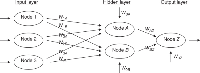
Figure 12.2 Simple neural network.
Single output nodes may also be used when the classes are clearly ordered. For example, suppose that we would like to classify elementary school reading prowess based on a certain set of student attributes. Then, we may be able to define the thresholds as follows:
- If 0 ≤ output < 0.25, classify first-grade reading level.
- If 0.25 ≤ output < 0.50, classify second-grade reading level.
- If 0.50 ≤ output < 0.75, classify third-grade reading level.
- If output
 0.75, classify fourth-grade reading level.
Fine-tuning of the thresholds may be required, tempered by the experience and the judgment of domain experts.
Not all classification problems, however, are soluble using a single output node only. For instance, suppose that we have several unordered categories in our target variable, as, for example, with the marital status variable mentioned above. In this case, we would choose to adopt 1-of-n output encoding, where one output node is used for each possible category of the target variable. For example, if marital status was our target variable, the network would have six output nodes in the output layer, one for each of the six classes divorced, married, separated, single, widowed, and unknown. The output node with the highest value is then chosen as the classification for that particular record.
One benefit of using 1-of-n output encoding is that it provides a measure of confidence in the classification, in the form of the difference between the highest-value output node and the second-highest-value output node. Classifications with low confidence (small difference in node output values) can be flagged for further clarification.
12.2 Neural Networks for Estimation and Prediction
Clearly, as neural networks produce continuous output, they may quite naturally be used for estimation and prediction. Suppose, for example, that we are interested in predicting the price of a particular stock 3 months in the future. Presumably, we would have encoded price information using the min–max normalization above. However, the neural network would output a value between 0 and 1, which (one would hope) does not represent the predicted price of the stock.
Rather, the min–max normalization needs to be inverted, so that the neural network output can be understood on the scale of the stock prices. In general, this denormalization is as follows:
where output represents the neural network output in the (0,1) range, data range represents the range of the original attribute values on the nonnormalized scale, and minimum represents the smallest attribute value on the nonnormalized scale. For example, suppose that the stock prices ranged from $20 to $30 and that the network output was 0.69. Then the predicted stock price in 3 months is
12.3 Simple Example of a Neural Network
Let us examine the simple neural network shown in Figure 12.2. A neural network consists of a layered, feedforward, completely connected network of artificial neurons, or nodes. The feedforward nature of the network restricts the network to a single direction of flow and does not allow looping or cycling. The neural network is composed of two or more layers, although most networks consist of three layers: an input layer, a hidden layer, and an output layer. There may be more than one hidden layer, however, most networks contain only one, which is sufficient for most purposes. The neural network is completely connected, meaning that every node in a given layer is connected to every node in the next layer, however, not to other nodes in the same layer. Each connection between nodes has a weight (e.g., W1A) associated with it. At initialization, these weights are randomly assigned to values between 0 and 1.
The number of input nodes usually depends on the number and type of attributes in the data set. The number of hidden layers and the number of nodes in each hidden layer are both configurable by the user. One may have more than one node in the output layer, depending on the particular classification task at hand.
How many nodes should one have in the hidden layer? As more nodes in the hidden layer increases the power and flexibility of the network for identifying complex patterns, one might be tempted to have a large number of nodes in the hidden layer. However, an overly large hidden layer leads to overfitting, memorizing the training set at the expense of generalizability to the validation set. If overfitting is occurring, one may consider reducing the number of nodes in the hidden layer; conversely, if the training accuracy is unacceptably low, one may consider increasing the number of nodes in the hidden layer.
The input layer accepts inputs from the data set, such as attribute values, and simply passes these values along to the hidden layer without further processing. Thus, the nodes in the input layer do not share the detailed node structure that the hidden layer nodes and the output layer nodes share.
We will investigate the structure of hidden layer nodes and output layer nodes using the sample data provided in Table 12.1. First, a combination function (usually summation, ∑) produces a linear combination of the node inputs and the connection weights into a single scalar value, which we will term as net. Thus, for a given node j,
where xij represents the ith input to node j, Wij represents the weight associated with the ith input to node j, and there are I + 1 inputs to node j. Note that x1, x2, …, xI represent inputs from upstream nodes, while x0 represents a constant input, analogous to the constant factor in regression models, which by convention uniquely takes the value x0j = 1. Thus, each hidden layer or output layer node j contains an “extra” input equal to a particular weight W0jx0j = W0j, such as W0B for node B.
Table 12.1 Data inputs and initial values for neural network weights
| x0 = 1.0 | W0A = 0.5 | W0B = 0.7 | W0Z = 0.5 |
| x1 = 0.4 | W1A = 0.6 | W1B = 0.9 | WAZ = 0.9 |
| x2 = 0.2 | W2A = 0.8 | W2B = 0.8 | WBZ = 0.9 |
| x3 = 0.7 | W3A = 0.6 | W3B = 0.4 |
For example, for node A in the hidden layer, we have

Within node A, this combination function netA = 1.32 is then used as an input to an activation function. In biological neurons, signals are sent between neurons when the combination of inputs to a particular neuron crosses a certain threshold, and the neuron “fires.” This is nonlinear behavior, as the firing response is not necessarily linearly related to the increment in input stimulation. Artificial neural networks model this behavior through a nonlinear activation function.
The most common activation function is the sigmoid function:
where e is base of natural logarithms, equal to about 2.718281828. Thus, within node A, the activation would take netA = 1.32 as input to the sigmoid activation function, and produce an output value of y = 1/(1 + e–1.32) = 0.7892. Node A's work is done (for the moment), and this output value would then be passed along the connection to the output node Z, where it would form (via another linear combination) a component of netZ.
But before we can compute netZ, we need to find the contribution of node B. From the values in Table 12.1, we have
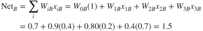
Then,
Node Z then combines these outputs from nodes A and B, through netZ, a weighted sum, using the weights associated with the connections between these nodes. Note that the inputs xi to node Z are not data attribute values but the outputs from the sigmoid functions from upstream nodes:

Finally, netZ is input into the sigmoid activation function in node Z, resulting in
This value of 0.8750 is the output from the neural network for this first pass through the network, and represents the value predicted for the target variable for the first observation.
12.4 Sigmoid Activation Function
Why use the sigmoid function? Because it combines nearly linear behavior, curvilinear behavior, and nearly constant behavior, depending on the value of the input. Figure 12.3 shows the graph of the sigmoid function y = f(x) = 1/(1 + e–x), for −5 < x < 5 (although f(x) may theoretically take any real-valued input). Through much of the center of the domain of the input x (e.g., −1 < x < 1), the behavior of f(x) is nearly linear. As the input moves away from the center, f(x) becomes curvilinear. By the time the input reaches extreme values, f(x) becomes nearly constant.

Figure 12.3 Graph of the sigmoid function y = f(x) = 1/(1 + e−x).
Moderate increments in the value of x produce varying increments in the value of f(x), depending on the location of x. Near the center, moderate increments in the value of x produce moderate increments in the value of f(x); however, near the extremes, moderate increments in the value of x produce tiny increments in the value of f(x). The sigmoid function is sometimes called a squashing function, as it takes any real-valued input and returns an output bounded between 0 and 1.
12.5 Back-Propagation
How does the neural network learn? Neural networks represent a supervised learning method, requiring a large training set of complete records, including the target variable. As each observation from the training set is processed through the network, an output value is produced from the output node (assuming that we have only one output node, as in Figure 12.2). This output value is then compared to the actual value of the target variable for this training set observation, and the error (actual − output) is calculated. This prediction error is analogous to the residuals in regression models. To measure how well the output predictions fit the actual target values, most neural network models use the sum of squared errors (SSE):
where the squared prediction errors are summed over all the output nodes and over all the records in the training set.
The problem is therefore to construct a set of model weights that will minimize the SSE. In this way, the weights are analogous to the parameters of a regression model. The “true” values for the weights that will minimize SSE are unknown, and our task is to estimate them, given the data. However, due to the nonlinear nature of the sigmoid functions permeating the network, there exists no closed-form solution for minimizing SSE as exists for least-squares regression.
12.6 Gradient-Descent Method
We must therefore turn to optimization methods, specifically gradient-descent methods, to help us find the set of weights that will minimize SSE. Suppose that we have a set (vector) of m weights w = w0, w1, w2, …, wm in our neural network model and we wish to find the values for each of these weights that, together, minimize SSE. We can use the gradient-descent method, which gives us the direction that we should adjust the weights in order to decrease SSE. The gradient of SSE with respect to the vector of weights w is the vector derivative:
that is, the vector of partial derivatives of SSE with respect to each of the weights.
To illustrate how gradientdescent works, let us consider the case where there is only a single weight w1. Consider Figure 12.4, which plots the error SSE against the range of values for w1. We would prefer values of w1 that would minimize the SSE. The optimal value for the weight w1 is indicated as ![]() . We would like to develop a rule that would help us move our current value of w1 closer to the optimal value
. We would like to develop a rule that would help us move our current value of w1 closer to the optimal value ![]() as follows: wnew = wcurrent + Δwcurrent, where Δwcurrent is the “change in the current location of w.”
as follows: wnew = wcurrent + Δwcurrent, where Δwcurrent is the “change in the current location of w.”
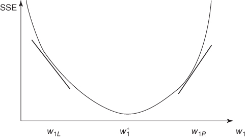
Figure 12.4 Using the slope of SSE with respect to w1 to find weight adjustment direction.
Now, suppose that our current weight value wcurrent is near w1L. Then we would like to increase our current weight value to bring it closer to the optimal value ![]() . However, if our current weight value wcurrent were near w1R, we would instead prefer to decrease its value, to bring it closer to the optimal value
. However, if our current weight value wcurrent were near w1R, we would instead prefer to decrease its value, to bring it closer to the optimal value ![]() . Now the derivative ∂SSE/∂w1 is simply the slope of the SSE curve at w1. For values of w1 close to w1L, this slope is negative, and for values of w1 close to w1R, this slope is positive. Hence, the direction for adjusting wcurrent is the negative of the sign of the derivative of SSE at wcurrent, that is, −sign(∂SSE/∂wcurrent).
. Now the derivative ∂SSE/∂w1 is simply the slope of the SSE curve at w1. For values of w1 close to w1L, this slope is negative, and for values of w1 close to w1R, this slope is positive. Hence, the direction for adjusting wcurrent is the negative of the sign of the derivative of SSE at wcurrent, that is, −sign(∂SSE/∂wcurrent).
Now, how far should wcurrent be adjusted in the direction of −sign(∂SSE/∂wcurrent)? Suppose that we use the magnitude of the derivative of SSE at wcurrent. When the curve is steep, the adjustment will be large, as the slope is greater in magnitude at those points. When the curve is nearly flat, the adjustment will be smaller, due to less slope. Finally, the derivative is multiplied by a positive constant η (Greek lowercase eta), called the learning rate, with values ranging between 0 and 1. (We discuss the role of η in more detail below.) The resulting form of Δwcurrent is as follows: Δwcurrent = −η(∂SSE/∂wcurrent), meaning that the change in the current weight value equals negative a small constant times the slope of the error function at wcurrent.
12.7 Back-Propagation Rules
The back-propagation algorithm takes the prediction error (actual − output) for a particular record and percolates the error back through the network, assigning partitioned responsibility for the error to the various connections. The weights on these connections are then adjusted to decrease the error using gradient descent.
Using the sigmoid activation function and gradient descent, Mitchell1 derives the back-propagation rules as follows:
Now we know that η represents the learning rate and xij signifies the ith input to node j, but what does δj represent? The component δj represents the responsibility for a particular error belonging to node j. The error responsibility is computed using the partial derivative of the sigmoid function with respect to netj and takes the following forms, depending on whether the node in question lies in the output layer or the hidden layer:

where ∑downstream Wjkδj refers to the weighted sum of the error responsibilities for the nodes downstream from the particular hidden layer node. (For the full derivation, see Mitchell.)
Also, note that the back-propagation rules illustrate why the attribute values need to be normalized to between 0 and 1. For example, if income data, with values ranging into six figures, were not normalized, the weight adjustment Δwij = ηδjxij would be dominated by the data value xij. Hence, the error propagation (in the form of δj) through the network would be overwhelmed, and learning (weight adjustment) would be stifled.
12.8 Example of Back-Propagation
Recall from our introductory example that the output from the first pass through the network was output = 0.8750. Assume that the actual value of the target attribute is actual = 0.8 and that we will use a learning rate of η = 0.1. Then the prediction error equals 0.8 − 0.8750 = −0.075, and we may apply the foregoing rules to illustrate how the back-propagation algorithm works to adjust the weights by portioning out responsibility for this error to the various nodes. Although it is possible to update the weights only after all records have been read, neural networks use stochastic (or online) back-propagation, which updates the weights after each record.
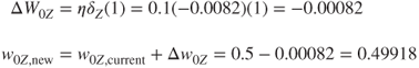
First, the error responsibility δZ for node Z is found. As node Z is an output node, we have
We may now adjust the “constant” weight W0Z (which transmits an “input” of 1) using the back-propagation rules as follows:
Next, we move upstream to node A. As node A is a hidden layer node, its error responsibility is
The only node downstream from node A is node Z. The weight associated with this connection is WAZ = 0.9, and the error responsibility at node Z is −0.0082, so that δA = 0.7892(1 − 0.7892)(0.9)(−0.0082) = −0.00123.
We may now update weight WAZ using the back-propagation rules as follows:
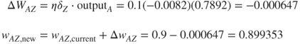
The weight for the connection between hidden layer node A and output layer node Z has been adjusted from its initial value of 0.9 to its new value of 0.899353.
Next, we turn to node B, a hidden layer node, with error responsibility
Again, the only node downstream from node B is node Z, giving us δB = 0.8176(1 − 0.8176)(0.9)(−0.0082) = −0.0011.
Weight WBZ may then be adjusted using the back-propagation rules as follows:

We move upstream to the connections being used as inputs to node A. For weight W1A we have

For weight W2A we have

For weight W3A we have

Finally, for weight W0A we have
Adjusting weights W0B, W1B, W2B, and W3B is left as an exercise.
Note that the weight adjustments have been made based on only a single perusal of a single record. The network calculated a predicted value for the target variable, compared this output value to the actual target value, and then percolated the error in prediction throughout the network, adjusting the weights to provide a smaller prediction error. Showing that the adjusted weights result in a smaller prediction error is left as an exercise.
12.9 Termination Criteria
The neural network algorithm would then proceed to work through the training data set, record by record, adjusting the weights constantly to reduce the prediction error. It may take many passes through the data set before the algorithm's termination criterion is met. What, then, serves as the termination criterion, or stopping criterion? If training time is an issue, one may simply set the number of passes through the data, or the amount of real time the algorithm may consume, as termination criteria. However, what one gains in short training time is probably bought with degradation in model efficacy.
Alternatively, one may be tempted to use a termination criterion that assesses when the SSE on the training data has been reduced to some low threshold level. Unfortunately, because of their flexibility, neural networks are prone to overfitting, memorizing the idiosyncratic patterns in the training set instead of retaining generalizability to unseen data.
Therefore, most neural network implementations adopt the following cross-validation termination procedure:
- Retain part of the original data set as a holdout validation set.
- Proceed to train the neural network as above on the remaining training data.
- Apply the weights learned from the training data on the validation data.
- Monitor two sets of weights, one “current” set of weights produced by the training data, and one “best” set of weights, as measured by the lowest SSE so far on the validation data.
- When the current set of weights has significantly greater SSE than the best set of weights, then terminate the algorithm.
Regardless of the stopping criterion used, the neural network is not guaranteed to arrive at the optimal solution, known as the global minimum for the SSE. Rather, the algorithm may become stuck in a local minimum, which represents a good, if not optimal solution. In practice, this has not presented an insuperable problem.
- For example, multiple networks may be trained using different initialized weights, with the best-performing model being chosen as the “final” model.
- Second, the online or stochastic back-propagation method itself acts as a guard against getting stuck in a local minimum, as it introduces a random element to the gradient descent (see Reed and Marks2).
- Alternatively, a momentum term may be added to the back-propagation algorithm, with effects discussed below.
12.10 Learning Rate
Recall that the learning rate η, 0 < η < 1, is a constant chosen to help us move the network weights toward a global minimum for SSE. However, what value should η take? How large should the weight adjustments be?
When the learning rate is very small, the weight adjustments tend to be very small. Thus, if η is small when the algorithm is initialized, the network will probably take an unacceptably long time to converge. Is the solution therefore to use large values for η? Not necessarily. Suppose that the algorithm is close to the optimal solution and we have a large value for η. This large η will tend to make the algorithm overshoot the optimal solution.
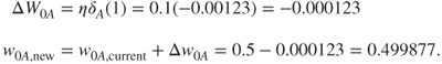
Consider Figure 12.5, where W* is the optimum value for weight W, which has current value Wcurrent. According to the gradient-descent rule, Δwcurrent = −η(∂SSE/∂wcurrent), Wcurrent will be adjusted in the direction of W*. But if the learning rate η, which acts as a multiplier in the formula for Δwcurrent, is too large, the new weight value Wnew will jump right past the optimal value W*, and may in fact end up farther away from W* than Wcurrent.
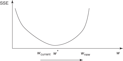
Figure 12.5 Large η may cause algorithm to overshoot global minimum.
In fact, as the new weight value will then be on the opposite side of W*, the next adjustment will again overshoot W*, leading to an unfortunate oscillation between the two “slopes” of the valley and never settling down in the ravine (the minimum). One solution is to allow the learning rate η to change values as the training moves forward. At the start of training, η should be initialized to a relatively large value to allow the network to quickly approach the general neighborhood of the optimal solution. Then, when the network is beginning to approach convergence, the learning rate should gradually be reduced, thereby avoiding overshooting the minimum.
12.11 Momentum Term
The back-propagation algorithm is made more powerful through the addition of a momentum term α, as follows:
where Δwprevious represents the previous weight adjustment, and 0 ≤ α < 1. Thus, the new component αΔwprevious represents a fraction of the previous weight adjustment for a given weight.
Essentially, the momentum term represents inertia. Large values of α will influence the adjustment in the current weight, Δwcurrent, to move in the same direction as previous adjustments. It has been shown (e.g., Reed and Marks) that including momentum in the back-propagation algorithm results in the adjustment becoming an exponential average of all previous adjustments:
The αk term indicates that the more recent adjustments exert a larger influence. Large values of α allow the algorithm to “remember” more terms in the adjustment history. Small values of α reduce the inertial effects as well as the influence of previous adjustments, until, with α = 0, the component disappears entirely.
Clearly, a momentum component will help to dampen the oscillations around optimality mentioned earlier, by encouraging the adjustments to stay in the same direction. But momentum also helps the algorithm in the early stages of the algorithm, by increasing the rate at which the weights approach the neighborhood of optimality. This is because these early adjustments will probably be all in the same direction, so that the exponential average of the adjustments will also be in that direction. Momentum is also helpful when the gradient of SSE with respect to w is flat. If the momentum term α is too large, then the weight adjustments may again overshoot the minimum, due to the cumulative influences of many previous adjustments.
For an informal appreciation of momentum, consider Figures 12.6 and 12.7. In both figures, the weight is initialized at location I, local minima exist at locations A and C, with the optimal global minimum at B. In Figure 12.6, suppose that we have a small value for the momentum term α, symbolized by the small mass of the “ball” on the curve. If we roll this small ball down the curve, it may never make it over the first hill, and remain stuck in the first valley. That is, the small value for α enables the algorithm to easily find the first trough at location A, representing a local minimum, but does not allow it to find the global minimum at B.

Figure 12.6 Small momentum α may cause algorithm to undershoot global minimum.

Figure 12.7 Large momentum α may cause algorithm to overshoot global minimum.
Next, in Figure 12.7, suppose that we have a large value for the momentum term α, symbolized by the large mass of the “ball” on the curve. If we roll this large ball down the curve, it may well make it over the first hill but may then have so much momentum that it overshoots the global minimum at location B and settles for the local minimum at location C.
Thus, one needs to consider carefully what values to set for both the learning rate η and the momentum term α. Experimentation with various values of η and α may be necessary before the best results are obtained.
12.12 Sensitivity Analysis
One of the drawbacks of neural networks is their opacity. The same wonderful flexibility that allows neural networks to model a wide range of nonlinear behavior also limits our ability to interpret the results using easily formulated rules. Unlike decision trees, no straightforward procedure exists for translating the weights of a neural network into a compact set of decision rules.
However, a procedure is available, called sensitivity analysis, which does allow us to measure the relative influence each attribute has on the output result. Using the test data set mentioned above, the sensitivity analysis proceeds as follows:
- Generate a new observation xmean, with each attribute value in xmean equal to the mean of the various attribute values for all records in the test set.
- Find the network output for input xmean. Call it outputmean.
- Attribute by attribute, vary xmean to reflect the attribute minimum and maximum. Find the network output for each variation and compare it to outputmean.
The sensitivity analysis will find that varying certain attributes from their minimum to their maximum will have a greater effect on the resulting network output than it has for other attributes. For example, suppose that we are interested in predicting stock price based on price to earnings ratio, dividend yield, and other attributes. Also, suppose that varying price to earnings ratio from its minimum to its maximum results in an increase of 0.20 in the network output, while varying dividend yield from its minimum to its maximum results in an increase of 0.30 in the network output when the other attributes are held constant at their mean value. We conclude that the network is more sensitive to variations in dividend yield and that therefore dividend yield is a more important factor for predicting stock prices than is price to earnings ratio.
12.13 Application of Neural Network Modeling
Next, we apply a neural network model using Insightful Miner on the adult data set from the UCal Irvine Machine Learning Repository. The Insightful Miner neural network software was applied to a training set of 25,000 cases, using a single hidden layer with eight hidden nodes. The algorithm iterated 47 epochs (runs through the data set) before termination. The resulting neural network is shown in Figure 12.8. The squares on the left represent the input nodes. For the categorical variables, there is one input node per class. The eight dark circles represent the hidden layer. The light gray circles represent the constant inputs. There is only a single output node, indicating whether or not the record is classified as having income less than or equal to $50,000.
Figure 12.8 Neural network for the adult data set generated by Insightful Miner.
In this algorithm, the weights are centered at 0. An excerpt of the computer output showing the weight values is provided in Figure 12.9. The columns in the first table represent the input nodes: 1 = age, 2 = education-num, and so on, while the rows represent the hidden layer nodes: 22 = first (top) hidden node, 23 = second hidden node, and so on. For example, the weight on the connection from age to the topmost hidden node is −0.97, while the weight on the connection from Race: American Indian/Eskimo (the sixth input node) to the last (bottom) hidden node is −0.75. The lower section of Figure 12.9 displays the weights from the hidden nodes to the output node.

Figure 12.9 Some of the neural network weights for the income example.
The estimated prediction accuracy using this very basic model is 82%, which is in the ballpark of the accuracies reported by Kohavi.3 As over 75% of the subjects have incomes at or below $50,000, simply predicted “less than or equal to $50,000” for every person would provide a baseline accuracy of about 75%.
However, we would like to know which variables are most important for predicting (classifying) income. We therefore perform a sensitivity analysis using Modeler, with results shown in Figure 12.10. Clearly, the amount of capital gains is the best predictor of whether a person has income less than or equal to $50,000, followed by the number of years of education. Other important variables include the number of hours worked per week and marital status. A person's gender does not seem to be highly predictive of income.
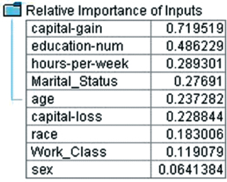
Figure 12.10 Most important variables: results from sensitivity analysis.
Of course, there is much more involved in developing a neural network classification model. For example, further data preprocessing may be called for; the model would need to be validated using a holdout validation data set, and so on. For a start-to-finish application of neural networks to a real-world data set, from data preparation through model building and sensitivity analysis, see the Case Study in Chapters 29–32.
R References
- 1 R Core Team. R: A Language and Environment for Statistical Computing. Vienna, Austria: R Foundation for Statistical Computing; 2012. ISBN: 3-900051-07-0, http://www.R-project.org/.
- 2 Venables WN, Ripley BD. Modern Applied Statistics with S. 4th ed. New York: Springer; 2002. ISBN: 0-387-95457-0.
Exercises
1. Suppose that you need to prepare the data in Table 6.10 for a neural network algorithm. Define the indicator variables for the occupation attribute.
2. Clearly describe each of these characteristics of a neural network:
- Layered
- Feedforward
- Completely connected
3. What is the sole function of the nodes in the input layer?
4. Should we prefer a large hidden layer or a small one? Describe the benefits and drawbacks of each.
5. Describe how neural networks function nonlinearly.
6. Explain why the updating term for the current weight includes the negative of the sign of the derivative (slope).
7. Adjust the weights W0B, W1B, W2B, and W3B from the example on back-propagation in the text.
8. Refer to Exercise 7. Show that the adjusted weights result in a smaller prediction error.
9. True or false: Neural networks are valuable because of their capacity for always finding the global minimum of the SSE.
10. Describe the benefits and drawbacks of using large or small values for the learning rate.
11. Describe the benefits and drawbacks of using large or small values for the momentum term.
Hands-On Analysis
For Exercises 12–14, use the data set churn. Normalize the numerical data, recode the categorical variables, and deal with the correlated variables.
12. Generate a neural network model for classifying churn based on the other variables. Describe the topology of the model.
13. Which variables, in order of importance, are identified as most important for classifying churn?
14. Compare the neural network model with the classification and regression tree (CART) and C4.5 models for this task in Chapter 11. Describe the benefits and drawbacks of the neural network model compared to the others. Is there convergence or divergence of results among the models?
For Exercises 15–17, use the ClassifyRisk data set.
15. Run a NN model predicting income based only on age. Use the default settings and make sure there is one hidden layer with one neuron.
16. Consider the following quantity: (weight for Age-to-Neuron1) + (weight for Bias-to-Neuron1)*(weight for Neuron 1-to-Output node). Explain whether this makes sense, given the data, and why.
17. Make sure the target variable takes the flag type. Compare the sign of (weight for Age-to-Neuron1) + (weight for Bias-to-Neuron1)*(weight for Neuron 1-to-Output node) for the good risk output node, as compared to the bad loss output node. Explain whether this makes sense, given the data, and why.
IBM/SPSS Modeler Analysis. For Exercises 18, 19, use the nn1 data set.
18. Set your neural network build options as follows: Use a Multilayer Perceptron and customize number of units in Hidden Layer 1 to be 1 and Hidden Layer 2 to be 0. For Stopping Rules, select ONLY Customize number of maximum training cycles. Start at 1 and go to about 20. For Advanced, de-select Replicate Results.
19. Browse your model. In the Network window of the Model tab, select the Style: Coefficients. Record the Pred1-to-Neuron1 weight and the Pred2-to-Neuron1 weight for each run. Describe the behavior of these weights. Explain why this is happening.