
Chapter 19
Hierarchical and k-Means Clustering
19.1 The Clustering Task
Clustering refers to the grouping of records, observations, or cases into classes of similar objects. A cluster is a collection of records that are similar to one another and dissimilar to records in other clusters. Clustering differs from classification in that there is no target variable for clustering. The clustering task does not try to classify, estimate, or predict the value of a target variable. Instead, clustering algorithms seek to segment the entire data set into relatively homogeneous subgroups or clusters, where the similarity of the records within the cluster is maximized, and the similarity to records outside this cluster is minimized.
For example, the Nielsen PRIZM segments, developed by Claritas Inc., represent demographic profiles of each geographic area in the United States, in terms of distinct lifestyle types, as defined by zip code. For example, the clusters identified for zip code 90210, Beverly Hills, California, are as follows:
- Cluster # 01: Upper Crust Estates
- Cluster # 03: Movers and Shakers
- Cluster # 04: Young Digerati
- Cluster # 07: Money and Brains
- Cluster # 16: Bohemian Mix.
The description for Cluster # 01: Upper Crust is “The nation's most exclusive address, Upper Crust is the wealthiest lifestyle in America, a haven for empty-nesting couples between the ages of 45 and 64. No segment has a higher concentration of residents earning over $100,000 a year and possessing a postgraduate degree. And none has a more opulent standard of living.”
Examples of clustering tasks in business and research include the following:
- Target marketing of a niche product for a small-capitalization business that does not have a large marketing budget.
- For accounting auditing purposes, to segment financial behavior into benign and suspicious categories.
- As a dimension-reduction tool when a data set has hundreds of attributes.
- For gene expression clustering, where very large quantities of genes may exhibit similar behavior.
Clustering is often performed as a preliminary step in a data mining process, with the resulting clusters being used as further inputs into a different technique downstream, such as neural networks. Owing to the enormous size of many present-day databases, it is often helpful to apply clustering analysis first, to reduce the search space for the downstream algorithms. In this chapter, after a brief look at hierarchical clustering methods, we discuss in detail k-means clustering; in Chapter 20, we examine clustering using Kohonen networks, a structure related to neural networks.
Cluster analysis encounters many of the same issues that we dealt with in the chapters on classification. For example, we shall need to determine
- how to measure similarity;
- how to recode categorical variables;
- how to standardize or normalize numerical variables;
- how many clusters we expect to uncover.
For simplicity, in this book, we concentrate on Euclidean distance between records:
where x = x1, x2, …, xm, and y = y1, y2, …, ym represent the m attribute values of two records. Of course, many other metrics exist, such as city-block distance:
or Minkowski distance, which represents the general case of the foregoing two metrics for a general exponent q:

For categorical variables, we may again define the “different from” function for comparing the ith attribute values of a pair of records:

where xi and yi are categorical values. We may then substitute different (xi, yi) for the ith term in the Euclidean distance metric above.
For optimal performance, clustering algorithms, just like algorithms for classification, require the data to be normalized so that no particular variable or subset of variables dominates the analysis. Analysts may use either the min–max normalization or Z-score standardization, discussed in earlier chapters:
All clustering methods have as their goal the identification of groups of records such that similarity within a group is very high while the similarity to records in other groups is very low. In other words, as shown in Figure 19.1, clustering algorithms seek to construct clusters of records such that the between-cluster variation is large compared to the within-cluster variation. This is somewhat analogous to the concept behind analysis of variance.
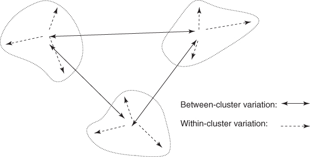
Figure 19.1 Clusters should have small within-cluster variation compared to the between-cluster variation.
19.2 Hierarchical Clustering Methods
Clustering algorithms are either hierarchical or nonhierarchical. In hierarchical clustering, a treelike cluster structure (dendrogram) is created through recursive partitioning (divisive methods) or combining (agglomerative) of existing clusters. Agglomerative clustering methods initialize each observation to be a tiny cluster of its own. Then, in succeeding steps, the two closest clusters are aggregated into a new combined cluster. In this way, the number of clusters in the data set is reduced by one at each step. Eventually, all records are combined into a single huge cluster. Divisive clustering methods begin with all the records in one big cluster, with the most dissimilar records being split off recursively, into a separate cluster, until each record represents its own cluster. Because most computer programs that apply hierarchical clustering use agglomerative methods, we focus on those.
Distance between records is rather straightforward once appropriate recoding and normalization has taken place. But how do we determine distance between clusters of records? Should we consider two clusters to be close if their nearest neighbors are close or if their farthest neighbors are close? How about criteria that average out these extremes?
We examine several criteria for determining distance between arbitrary clusters A and B:
- Single linkage, sometimes termed the nearest-neighbor approach, is based on the minimum distance between any record in cluster A and any record in cluster B. In other words, cluster similarity is based on the similarity of the most similar members from each cluster. Single linkage tends to form long, slender clusters, which may sometimes lead to heterogeneous records being clustered together.
- Complete linkage, sometimes termed the farthest-neighbor approach, is based on the maximum distance between any record in cluster A and any record in cluster B. In other words, cluster similarity is based on the similarity of the most dissimilar members from each cluster. Complete linkage tends to form more compact, spherelike clusters.
- Average linkage is designed to reduce the dependence of the cluster-linkage criterion on extreme values, such as the most similar or dissimilar records. In average linkage, the criterion is the average distance of all the records in cluster A from all the records in cluster B. The resulting clusters tend to have approximately equal within-cluster variability.
Let us examine how these linkage methods work, using the following small, one-dimensional data set:
| 2 | 5 | 9 | 15 | 16 | 18 | 25 | 33 | 33 | 45 |
19.3 Single-Linkage Clustering
Suppose that we are interested in using single-linkage agglomerative clustering on this data set. Agglomerative methods start by assigning each record to its own cluster. Then, single linkage seeks the minimum distance between any records in two clusters. Figure 19.2 illustrates how this is accomplished for this data set. The minimum cluster distance is clearly between the single-record clusters where each contains the value 33, for which the distance must be 0 for any valid metric. Thus, these two clusters are combined into a new cluster of two records, both of value 33, as shown in Figure 19.2. Note that, after step 1, only nine (n − 1) clusters remain. Next, in step 2, the clusters containing values 15 and 16 are combined into a new cluster, because their distance of 1 is the minimum between any two clusters remaining.
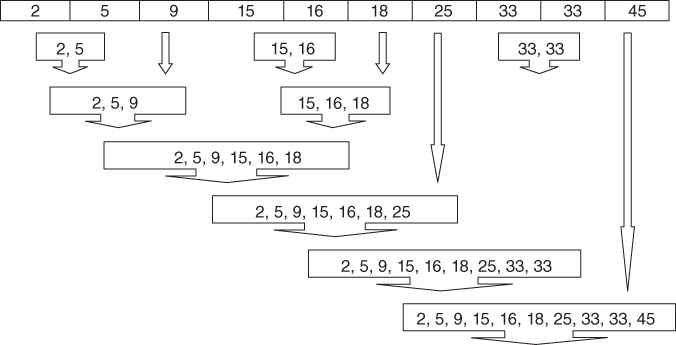
Figure 19.2 Single-linkage agglomerative clustering on the sample data set.
Here are the remaining steps:
- Step 3: The cluster containing values 15 and 16 (cluster {15,16}) is combined with cluster {18}, because the distance between 16 and 18 (the closest records in each cluster) is 2, the minimum among remaining clusters.
- Step 4: Clusters {2} and {5} are combined.
- Step 5: Cluster {2,5} is combined with cluster {9}, because the distance between 5 and 9 (the closest records in each cluster) is 4, the minimum among remaining clusters.
- Step 6: Cluster {2,5,9} is combined with cluster {15,16,18}, because the distance between 9 and 15 is 6, the minimum among remaining clusters.
- Step 7: Cluster {2,5,9,15,16,18} is combined with cluster {25}, because the distance between 18 and 25 is 7, the minimum among remaining clusters.
- Step 8: Cluster {2,5,9,15,16,18,25} is combined with cluster {33,33}, because the distance between 25 and 33 is 8, the minimum among remaining clusters.
- Step 9: Cluster {2,5,9,15,16,18,25,33,33} is combined with cluster {45}. This last cluster now contains all the records in the data set.
19.4 Complete-Linkage Clustering
Next, let us examine whether using the complete-linkage criterion would result in a different clustering of this sample data set. Complete linkage seeks to minimize the distance among the records in two clusters that are farthest from each other. Figure 19.3 illustrates complete-linkage clustering for this data set.
- Step 1: As each cluster contains a single record only, there is no difference between single linkage and complete linkage at step 1. The two clusters each containing 33 are again combined.
- Step 2: Just as for single linkage, the clusters containing values 15 and 16 are combined into a new cluster. Again, this is because there is no difference in the two criteria for single-record clusters.
- Step 3: At this point, complete linkage begins to diverge from its predecessor. In single linkage, cluster {15,16} was at this point combined with cluster {18}. But complete linkage looks at the farthest neighbors, not the nearest neighbors. The farthest neighbors for these two clusters are 15 and 18, for a distance of 3. This is the same distance separating clusters {2} and {5}. The complete-linkage criterion is silent regarding ties, so we arbitrarily select the first such combination found, therefore combining the clusters {2} and {5} into a new cluster.
- Step 4: Now cluster {15,16} is combined with cluster {18}.
- Step 5: Cluster {2,5} is combined with cluster {9}, because the complete-linkage distance is 7, the smallest among remaining clusters.
- Step 6: Cluster {25} is combined with cluster {33,33}, with a complete-linkage distance of 8.
- Step 7: Cluster {2,5,9} is combined with cluster {15,16,18}, with a complete-linkage distance of 16.
- Step 8: Cluster {25,33,33} is combined with cluster {45}, with a complete-linkage distance of 20.
- Step 9: Cluster {2,5,9,15,16,18} is combined with cluster {25,33,33,45}. All records are now contained in this last large cluster.
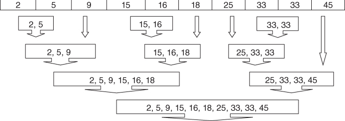
Figure 19.3 Complete-linkage agglomerative clustering on the sample data set.
Finally, with average linkage, the criterion is the average distance of all the records in cluster A from all the records in cluster B. As the average of a single record is the record's value itself, this method does not differ from the earlier methods in the early stages, where single-record clusters are being combined. At step 3, average linkage would be faced with the choice of combining clusters {2} and {5}, or combining the {15,16} cluster with the single-record {18} cluster. The average distance between the {15,16} cluster and the {18} cluster is the average of |18 − 15| and |18 − 16|, which is 2.5, while the average distance between clusters {2} and {5} is of course 3. Therefore, average linkage would combine the {15,16} cluster with cluster {18} at this step, followed by combining cluster {2} with cluster {5}. The reader may verify that the average-linkage criterion leads to the same hierarchical structure for this example as the complete-linkage criterion. In general, average linkage leads to clusters more similar in shape to complete linkage than does single linkage.
19.5 -Means Clustering
The k-means clustering algorithm1 is a straightforward and effective algorithm for finding clusters in data. The algorithm proceeds as follows:
- Step 1: Ask the user how many clusters k the data set should be partitioned into.
- Step 2: Randomly assign k records to be the initial cluster center locations.
- Step 3: For each record, find the nearest cluster center. Thus, in a sense, each cluster center “owns” a subset of the records, thereby representing a partition of the data set. We therefore have k clusters, C1, C2, …, Ck.
- Step 4: For each of the k clusters, find the cluster centroid, and update the location of each cluster center to the new value of the centroid.
- Step 5: Repeat steps 3–5 until convergence or termination.
The “nearest” criterion in step 3 is usually Euclidean distance, although other criteria may be applied as well. The cluster centroid in step 4 is found as follows. Suppose that we have n data points (a1, b1, c1), (a2, b2, c2), …, (an, bn, cn), the centroid of these points is the center of gravity of these points and is located at point ![]() . For example, the points (1,1,1), (1,2,1), (1,3,1), and (2,1,1) would have centroid
. For example, the points (1,1,1), (1,2,1), (1,3,1), and (2,1,1) would have centroid
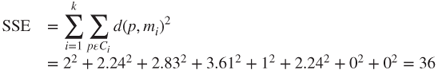
The algorithm terminates when the centroids no longer change. In other words, the algorithm terminates when for all clusters C1, C2, …, Ck, all the records “owned” by each cluster center remain in that cluster. Alternatively, the algorithm may terminate when some convergence criterion is met, such as no significant shrinkage in the mean squared error (MSE):
where SSE represents the sum of squares error, p ∈ Ci represents each data point in cluster i, mi represents the centroid (cluster center) of cluster i, N is the total sample size, and k is the number of clusters. Recall that clustering algorithms seek to construct clusters of records such that the between-cluster variation is large compared to the within-cluster variation. Because this concept is analogous to the analysis of variance, we may define a pseudo-F statistic as follows:
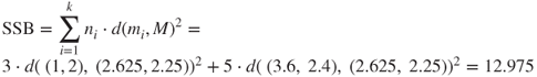
where SSE is defined as above, MSB is the mean square between, and SSB is the sum of squares between clusters, defined as

where ![]() is the number of records in cluster i,
is the number of records in cluster i, ![]() is the centroid (cluster center) for cluster i, and M is the grand mean of all the data.
is the centroid (cluster center) for cluster i, and M is the grand mean of all the data.
MSB represents the between-cluster variation and MSE represents the within-cluster variation. Thus, a “good” cluster would have a large value of the pseudo-F statistic, representing a situation where the between-cluster variation is large compared to the within-cluster variation. Hence, as the k-means algorithm proceeds, and the quality of the clusters increases, we would expect MSB to increase, MSE to decrease, and F to increase.
19.6 Example of -Means Clustering at Work
Let us examine an example of how the k-means algorithm works. Suppose that we have the eight data points in two-dimensional space shown in Table 19.1 and plotted in Figure 19.4 and are interested in uncovering k = 2 clusters.
Table 19.1 Data points for k-means example
| a | b | c | d | e | f | g | h |
| (1,3) | (3,3) | (4,3) | (5,3) | (1,2) | (4,2) | (1,1) | (2,1) |
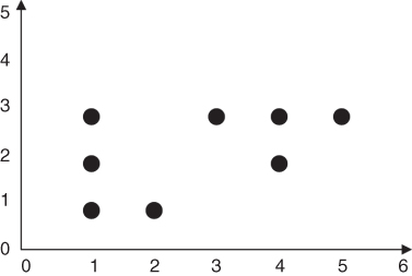
Figure 19.4 How will k-means partition this data into k = 2 clusters?
Let us apply the k-means algorithm step by step.
- Step 1: Ask the user how many clusters k the data set should be partitioned into. We have already indicated that we are interested in k = 2 clusters.
- Step 2: Randomly assign k records to be the initial cluster center locations. For this example, we assign the cluster centers to be m1 = (1,1) and m2 = (2,1).
- Step 3 (first pass): For each record, find the nearest cluster center. Table 19.2 contains the (rounded) Euclidean distances between each point and each cluster center m1 = (1,1) and m2 = (2,1), along with an indication of which cluster center the point is nearest to. Therefore, cluster 1 contains points {a,e,g}, and cluster 2 contains points {b,c,d,f,h}.
- Step 4 (first pass): For each of the k clusters find the cluster centroid and update the location of each cluster center to the new value of the centroid. The centroid for cluster 1 is [(1 + 1 + 1)/3, (3 + 2 + 1)/3] = (1,2). The centroid for cluster 2 is [(3 + 4 + 5 + 4 + 2)/5, (3 + 3 + 3 + 2 + 1)/5] = (3.6, 2.4). The clusters and centroids (triangles) at the end of the first pass are shown in Figure 19.5. Note that m1 has moved up to the center of the three points in cluster 1, while m2 has moved up and to the right a considerable distance, to the center of the five points in cluster 2.
- Step 5: Repeat steps 3 and 4 until convergence or termination. The centroids have moved, so we go back to step 3 for our second pass through the algorithm.
- Step 3 (second pass): For each record, find the nearest cluster center. Table 19.3 shows the distances between each point and each updated cluster center m1 = (1,2) and m2 = (3.6, 2.4), together with the resulting cluster membership. There has been a shift of a single record (h) from cluster 2 to cluster 1. The relatively large change in m2 has left record h now closer to m1 than to m2, so that record h now belongs to cluster 1. All other records remain in the same clusters as previously. Therefore, cluster 1 is {a,e,g,h}, and cluster 2 is {b,c,d,f}.
Table 19.2 Finding the nearest cluster center for each record (first pass)
| Point | Distance from m1 | Distance from m2 | Cluster Membership |
| a | 2.00 | 2.24 | C1 |
| b | 2.83 | 2.24 | C2 |
| c | 3.61 | 2.83 | C2 |
| d | 4.47 | 3.61 | C2 |
| e | 1.00 | 1.41 | C1 |
| f | 3.16 | 2.24 | C2 |
| g | 0.00 | 1.00 | C1 |
| h | 1.00 | 0.00 | C2 |
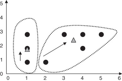
Figure 19.5 Clusters and centroids Δ after first pass through k-means algorithm.
Table 19.3 Finding the nearest cluster center for each record (second pass)
| Point | Distance from m1 | Distance from m2 | Cluster Membership |
| a | 1.00 | 2.67 | C1 |
| b | 2.24 | 0.85 | C2 |
| c | 3.16 | 0.72 | C2 |
| d | 4.12 | 1.52 | C2 |
| e | 0.00 | 2.63 | C1 |
| f | 3.00 | 0.57 | C2 |
| g | 1.00 | 2.95 | C1 |
| h | 1.41 | 2.13 | C1 |
- Step 4 (second pass): For each of the k clusters, find the cluster centroid and update the location of each cluster center to the new value of the centroid. The new centroid for cluster 1 is [(1 + 1 + 1 + 2)/4, (3 + 2 + 1 + 1)/4] = (1.25, 1.75). The new centroid for cluster 2 is [(3 + 4 + 5 + 4)/4, (3 + 3 + 3 + 2)/4] =(4, 2.75). The clusters and centroids at the end of the second pass are shown in Figure 19.6. Centroids m1 and m2 have both moved slightly.
- Step 5: Repeat steps 3 and 4 until convergence or termination. As the centroids have moved, we once again return to step 3 for our third (and as it turns out, final) pass through the algorithm.
- Step 3 (third pass): For each record, find the nearest cluster center. Table 19.4 shows the distances between each point and each newly updated cluster center m1 = (1.25, 1.75) and m2 = (4, 2.75), together with the resulting cluster membership. Note that no records have shifted cluster membership from the preceding pass.
- Step 4 (third pass): For each of the k clusters, find the cluster centroid and update the location of each cluster center to the new value of the centroid. As no records have shifted cluster membership, the cluster centroids therefore also remain unchanged.
- Step 5: Repeat steps 3 and 4 until convergence or termination. As the centroids remain unchanged, the algorithm terminates.
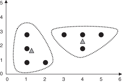
Figure 19.6 Clusters and centroids Δ after second pass through k-means algorithm.
Table 19.4 Finding the nearest cluster center for each record (third pass)
| Point | Distance from m1 | Distance from m2 | Cluster Membership |
| a | 1.27 | 3.01 | C1 |
| b | 2.15 | 1.03 | C2 |
| c | 3.02 | 0.25 | C2 |
| d | 3.95 | 1.03 | C2 |
| e | 0.35 | 3.09 | C1 |
| f | 2.76 | 0.75 | C2 |
| g | 0.79 | 3.47 | C1 |
| h | 1.06 | 2.66 | C1 |
19.7 Behavior of MSB, MSE, and Pseudo-F as the -Means Algorithm Proceeds
Let us observe the behavior of these statistics after step 4 of each pass.
First pass:
In general, we would expect MSB to increase, MSE to decrease, and F to increase, and such is the case. The calculations are left as an exercise.
These statistics indicate that we have achieved the maximum between-cluster variation (as measured by MSB), compared to the within-cluster variation (as measured by MSE).
Note that the k-means algorithm cannot guarantee finding the global maximum pseudo-F statistic, instead often settling at a local maximum. To improve the probability of achieving a global minimum, the analyst may consider using a variety of initial cluster centers. Moore1 suggests (i) placing the first cluster center on a random data point, and (ii) placing the subsequent cluster centers on points as far away from previous centers as possible.
One potential problem for applying the k-means algorithm is: Who decides how many clusters to search for? That is, who decides k? Unless the analyst has a priori knowledge of the number of underlying clusters; therefore, an “outer loop” should be added to the algorithm, which cycles through various promising values of k. Clustering solutions for each value of k can therefore be compared, with the value of k resulting in the largest F statistic being selected. Alternatively, some clustering algorithms, such as the BIRCH clustering algorithm, can select the optimal number of clusters.2
What if some attributes are more relevant than others to the problem formulation? As cluster membership is determined by distance, we may apply the same axis-stretching methods for quantifying attribute relevance that we discussed in Chapter 10. In Chapter 20, we examine another common clustering method, Kohonen networks, which are related to artificial neural networks in structure.
19.8 Application of -Means Clustering Using SAS Enterprise Miner
Next, we turn to the powerful SAS Enterpriser Miner3 software for an application of the k-means algorithm on the churn data set (available at the book series web site; also available from http://www.sgi.com/tech/mlc/db/). Recall that the data set contains 20 variables' worth of information about 3333 customers, along with an indication of whether or not that customer churned (left the company).
The following variables were passed to the Enterprise Miner clustering node:
- Flag (0/1) variables
- International Plan and VoiceMail Plan
- Numerical variables
- Account length, voice mail messages, day minutes, evening minutes, night minutes, international minutes, and customer service calls
- After applying min–max normalization to all numerical variables.
The Enterprise Miner clustering node uses SAS's FASTCLUS procedure, a version of the k-means algorithm. The number of clusters was set to k = 3. The three clusters uncovered by the algorithm varied greatly in size, with tiny cluster 1 containing 92 records, large cluster 2 containing 2411 records, and medium-sized cluster 3 containing 830 records.
Some basic cluster profiling will help us to learn about the types of records falling into each cluster. Figure 19.7 provides a look at the clustering results window of Enterprise Miner, containing a pie chart profile of the International Plan membership across the three clusters. All members of cluster 1, a fraction of the members of cluster 2, and no members of cluster 3 have adopted the International Plan. Note that the leftmost pie chart represents all records, and is similar to cluster 2.
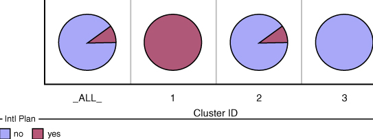
Figure 19.7 Enterprise Miner profile of International Plan adopters across clusters.
Next, Figure 19.8 illustrates the proportion of VoiceMail Plan adopters in each cluster. (Note the confusing color reversal for yes/no responses.) Remarkably, clusters 1 and 3 contain only VoiceMail Plan adopters, while cluster 2 contains only nonadopters of the plan. In other words, this field was used by the k-means algorithm to create a “perfect” discrimination, dividing the data set perfectly among adopters and nonadopters of the International Plan.

Figure 19.8 VoiceMail Plan adopters and nonadopters are mutually exclusive.
It is clear from these results that the algorithm is relying heavily on the categorical variables to form clusters. The comparison of the means of the numerical variables across the clusters in Table 19.5 shows relatively little variation, indicating that the clusters are similar across these dimensions. Figure 19.9, for example, illustrates that the distribution of customer service calls (normalized) is relatively similar in each cluster. If the analyst is not comfortable with this domination of the clustering by the categorical variables, he or she can choose to stretch or shrink the appropriate axes, as mentioned earlier, which will help to adjust the clustering algorithm to a more suitable solution.
Table 19.5 Comparison of variable means across clusters shows little variation
| Cluster | Frequency | AcctLength_m | VMailMessage | DayMins_mm |
| 1 | 92 | 0.4340639598 | 0.5826939471 | 0.5360015616 |
| 2 | 2411 | 0.4131940041 | 0 | 0.5126334451 |
| 3 | 830 | 0.4120730857 | 0.5731159934 | 0.5093940185 |
| Cluster | EveMins_mm | NightMins_mm | IntMins_mm | CustServCalls |
| 1 | 0.5669029659 | 0.4764366069 | 0.5467934783 | 0.1630434783 |
| 2 | 0.5507417372 | 0.4773586813 | 0.5119784322 | 0.1752615328 |
| 3 | 0.5564095259 | 0.4795138596 | 0.5076626506 | 0.1701472557 |

Figure 19.9 Distribution of customer service calls is similar across clusters.
The clusters may therefore be summarized, using only the categorical variables, as follows:
- Cluster 1: Sophisticated Users. A small group of customers who have adopted both the International Plan and the VoiceMail Plan.
- Cluster 2: The Average Majority. The largest segment of the customer base, some of whom have adopted the VoiceMail Plan but none of whom have adopted the International Plan.
- Cluster 3: Voice Mail Users. A medium-sized group of customers who have all adopted the VoiceMail Plan but not the International Plan.
19.9 Using Cluster Membership to Predict Churn
Suppose, however, that we would like to apply these clusters to assist us in the churn classification task. We may compare the proportions of churners directly among the various clusters, using graphs such as Figure 19.10. Here we see that overall (the leftmost column of pie charts), the proportion of churners is much higher among those who have adopted the International Plan than among those who have not. This finding was uncovered in Chapter 3. Note that the churn proportion is higher in cluster 1, which contains International Plan adopters, than in cluster 2, which contains a mixture of adopters and nonadopters, and higher still than cluster 3, which contains no such adopters of the International Plan. Clearly, the company should look at the plan to see why the customers who have it are leaving the company at a higher rate.

Figure 19.10 Churn behavior across clusters for International Plan adopters and nonadopters.
Now, as we know from Chapter 3 that the proportion of churners is lower among adopters of the VoiceMail Plan, we would expect that the churn rate for cluster 3 would be lower than for the other clusters. This expectation is confirmed in Figure 19.11.

Figure 19.11 Churn behavior across clusters for VoiceMail Plan adopters and nonadopters.
In Chapter 20, we explore using cluster membership as input to downstream data mining models.
R References
- Maechler M, Rousseeuw P, Struyf A, Hubert M, Hornik K. 2013. cluster: Cluster analysis basics and extensions. R package version 1.14.4.
- R Core Team. R: A Language and Environment for Statistical Computing. Vienna, Austria: R Foundation for Statistical Computing; 2012. ISBN: 3-900051-07-0, http://www.R-project.org/. Accessed 2014 Sep 30.
Exercises
Clarifying the Concepts
1. To which cluster for the 90210 zip code would you prefer to belong?
2. Describe the goal of all clustering methods.
3. Suppose that we have the following data (one variable). Use single linkage to identify the clusters. Data:
| 0 | 0 | 1 | 3 | 3 | 6 | 7 | 9 | 10 | 10 |
4. Suppose that we have the following data (one variable). Use complete linkage to identify the clusters. Data:
| 0 | 0 | 1 | 3 | 3 | 6 | 7 | 9 | 10 | 10 |
5. What is an intuitive idea for the meaning of the centroid of a cluster?
6. Suppose that we have the following data:
| a | b | c | d | e | f | g | h | i | j |
| (2,0) | (1,2) | (2,2) | (3,2) | (2,3) | (3,3) | (2,4) | (3,4) | (4,4) | (3,5) |
Identify the cluster by applying the k-means algorithm, with k = 2. Try using initial cluster centers as far apart as possible.
7. Refer to Exercise 6. Show that the ratio of the between-cluster variation to the within-cluster variation increases with each pass of the algorithm.
8. Once again identify the clusters in Exercise 6 data, this time by applying the k-means algorithm, with k = 3. Try using initial cluster centers as far apart as possible.
9. Refer to Exercise 8. Show that the ratio of the between-cluster variation to the within-cluster variation increases with each pass of the algorithm.
10. Which clustering solution do you think is preferable? Why?
11. Confirm the calculations for the second pass and third pass for MSB, MSE, and pseudo-F for step 4 of the example given in the chapter.
Hands-On Analysis
Use the cereals data set, included at the book series web site, for the following exercises. Make sure that the data are normalized.
12. Using all of the variables, except name and rating, run the k-means algorithm with k = 5 to identify clusters within the data.
13. Develop clustering profiles that clearly describe the characteristics of the cereals within the cluster.
14. Rerun the k-means algorithm with k = 3.
15. Which clustering solution do you prefer, and why?
16. Develop clustering profiles that clearly describe the characteristics of the cereals within the cluster.
17. Use cluster membership to predict rating. One way to do this would be to construct a histogram of rating based on cluster membership alone. Describe how the relationship you uncovered makes sense, based on your earlier profiles.