
Chapter 21
BIRCH Clustering
21.1 Rationale for BIRCH Clustering
BIRCH, which stands for Balanced Iterative Reducing and Clustering using Hierarchies, was developed in 1996 by Tian Zhang, Raghu Ramakrishnan, and Miron Livny.1 BIRCH is especially appropriate for very large data sets, or for streaming data, because of its ability to find a good clustering solution with only a single scan of the data. Optionally, the algorithm can make further scans through the data to improve the clustering quality. BIRCH handles large data sets with a time complexity and space efficiency that is superior to other algorithms, according to the authors.
The BIRCH clustering algorithm consists of two main phases or steps,2 as shown here.
BIRCH is sometimes referred to as Two-Step Clustering, because of the two phases shown here. We now consider what constitutes each of these phases.
21.2 Cluster Features
BIRCH clustering achieves its high efficiency by clever use of a small set of summary statistics to represent a larger set of data points. For clustering purposes, these summary statistics constitute a CF, and represent a sufficient substitute for the actual data. In their original paper, Zhang et al. suggested the following summary statistics for the CF:
For example, consider Clusters 1 and 2 in Figure 21.1. Cluster 1 contains data values (1, 1), (2, 1), and (1, 2), whereas Cluster 2 contains data values (3, 2), (4, 1), and (4, 2). ![]() , the CF for Cluster 1, consists of the following:
, the CF for Cluster 1, consists of the following:

And for Cluster 2, the CF is

![]() and
and ![]() represent the data in Clusters 1 and 2.
represent the data in Clusters 1 and 2.

Figure 21.1 Clusters 1 and 2.
One mechanism of the BIRCH algorithm calls for the merging of clusters under certain conditions. The Additivity Theorem states that the CFs for two clusters may be merged simply by adding the items in their respective CF trees. Thus, if we needed to merge Clusters 1 and 2, the resulting CF would be
21.3 Cluster Feature TREE
A CF tree is a tree structure composed of CFs. A CF tree represents a compressed form of the data, preserving any clustering structure in the data. A CF tree has the following parameters:
The general structure of a CF tree is shown in Figure 21.2.
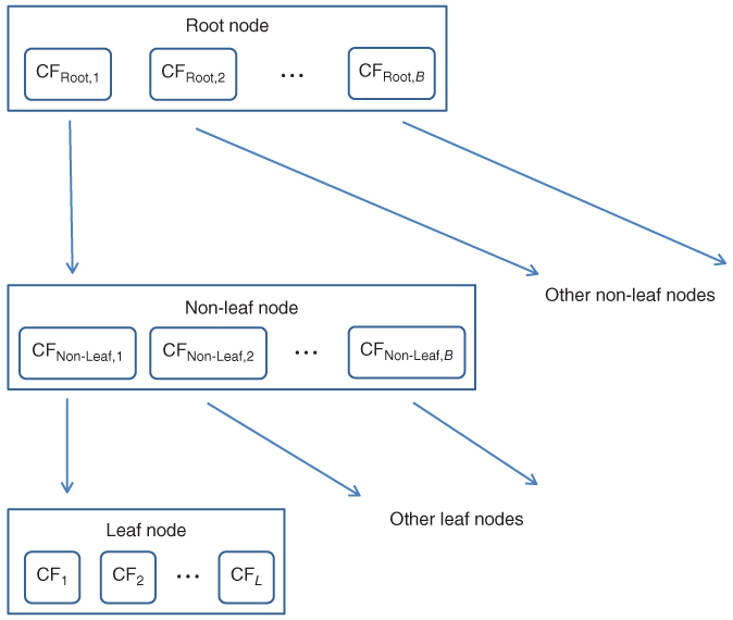
Figure 21.2 General structure of a CF tree, with branching factor B, and L leafs in each leaf node.
For a CF entry in a root node or a non-leaf node, that CF entry equals the sum of the CF entries in the child nodes of that entry. A leaf node CF is referred to simply as a leaf.
21.4 Phase 1: Building The CF Tree
Phase 1 of the BIRCH algorithm consists of building the CF tree. This is done using a sequential clustering approach, whereby the algorithm scans the data one record at a time, and determines whether a given record should be assigned to an existing cluster, or a new cluster should be constructed. The CF tree building process consists of four steps, as follows:
Now, if step 4b is executed, and there are already the maximum of L leafs in the leaf node, then the leaf node is split into two leaf nodes. The most distant leaf node CFs are used as leaf node seeds, with the remaining CFs being assigned to whichever leaf node is closer. If the parent node is full, split the parent node, and so on. This process is illustrated in the example below.
Each leaf node CF may be viewed as a sub-cluster. In the cluster step, these sub-clusters will be combined into clusters. For a given cluster, let the cluster centroid be
Then the radius of the cluster is
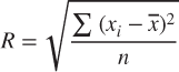
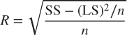
Note that the radius of a cluster may be calculated even without knowing the data points, as long as we have the count n, the linear sum LS, and the squared sum SS. This allows BIRCH to evaluate whether a given data point belongs to a particular sub-cluster without needing to scan the original data set. The derivation for the sum of squares is as follows:

Then,
The Threshold T allows the CF tree to be resized when it grows too big, that is, when B or L are exceeded. In such a case, T may be increased, allowing more records to be assigned to the individual CFs, thereby reducing the overall size of the CF tree, and allowing more records to be input.
21.5 Phase 2: Clustering The Sub-Clusters
Once the CF tree is built, any existing clustering algorithm may be applied to the sub-clusters (the CF leaf nodes), to combine these sub-clusters into clusters. For example, in their original paper presenting BIRCH clustering, the authors used agglomerative hierarchical clustering3 for the cluster step, as does IBM/SPSS Modeler. Because there are many fewer sub-clusters than data records, the task becomes much easier for the clustering algorithm in the cluster step.
As mentioned earlier, BIRCH clustering achieves its high efficiency by substituting a small set of summary statistics to represent a larger set of data points. When a new data value is added, these statistics may be easily updated. Because of this, the CF tree is much smaller than the original data set, allowing for more efficient computation.
A detriment of BIRCH clustering is the following. Because of the tree structure inherent in the CF tree, the clustering solution may be dependent on the input ordering of the data records. To avoid this, the data analyst may wish to apply BIRCH clustering on a few different random sortings of the data, and find consensus among the results.
However, a benefit of BIRCH clustering is that the analyst is not required to select the best choice of k, the number of clusters, as is the case with some other clustering methods. Rather, the number of clusters in a BIRCH clustering solution is an outcome of the tree-building process. (See later in the chapter for more on choosing the number of clusters with BIRCH.)
21.6 Example of Birch Clustering, Phase 1: Building The CF Tree
Let us examine in detail the workings of the BIRCH clustering algorithm as applied to the following one-dimensional toy data set.4
Let us define our CF tree parameters as follows:
- Threshold T = 0.15; no leaf may exceed 0.15 in radius.
- Number of entries in a leaf node L = 2.
- Branching factor B = 2; maximum number of child nodes for each non-leaf node.
The first data value ![]() is entered. The root node is initialized with the CF values of the first data value. A new leaf
is entered. The root node is initialized with the CF values of the first data value. A new leaf ![]() is created, and BIRCH assigns the first record
is created, and BIRCH assigns the first record ![]() to
to ![]() . Because it contains only one record, the radius of
. Because it contains only one record, the radius of ![]() is zero, and thus less than T = 0.15. The CF tree after one record is shown in Figure 21.3.
is zero, and thus less than T = 0.15. The CF tree after one record is shown in Figure 21.3.

Figure 21.3 CF Tree after the first data value is entered.
The second data value ![]() is entered. BIRCH tentatively passes
is entered. BIRCH tentatively passes ![]() to
to ![]() . The radius of
. The radius of ![]() is now
is now ![]() , so
, so ![]() is assigned to
is assigned to ![]() . The summary statistics for
. The summary statistics for ![]() are then updated as shown in Figure 21.4.
are then updated as shown in Figure 21.4.
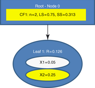
Figure 21.4 Second data value entered: Summary statistics are updated.
The third data value ![]() is entered. BIRCH tentatively passes
is entered. BIRCH tentatively passes ![]() to
to ![]() . However, the radius of
. However, the radius of ![]() now increases to
now increases to ![]() . The Threshold value
. The Threshold value ![]() is exceeded, so
is exceeded, so ![]() is not assigned to
is not assigned to ![]() . Instead, a new leaf is initialized, called
. Instead, a new leaf is initialized, called ![]() , containing
, containing ![]() only. The summary statistics for
only. The summary statistics for ![]() and
and ![]() are shown in Figure 21.5.
are shown in Figure 21.5.
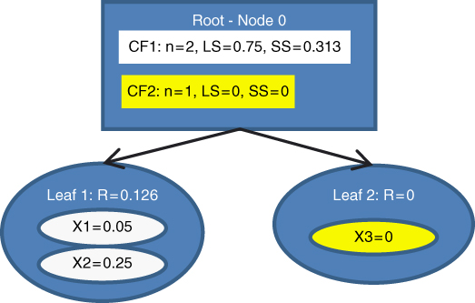
Figure 21.5 Third data value entered: A new leaf is initialized.
The fourth data value ![]() is entered. BIRCH compares
is entered. BIRCH compares ![]() to the locations of
to the locations of ![]() and CF2. The location is measured by
and CF2. The location is measured by ![]() . We have
. We have ![]() and
and ![]() . The data point
. The data point ![]() is thus closer to CF1 than to CF2. BIRCH tentatively passes
is thus closer to CF1 than to CF2. BIRCH tentatively passes ![]() to CF1. The radius of CF1 now increases to
to CF1. The radius of CF1 now increases to ![]() . The Threshold value
. The Threshold value ![]() is exceeded, so
is exceeded, so ![]() is not assigned to CF1. Instead, we would like to initialize a new leaf. However, L = 2 means that we cannot have three leafs in a leaf node. We must therefore split the root node into (i)
is not assigned to CF1. Instead, we would like to initialize a new leaf. However, L = 2 means that we cannot have three leafs in a leaf node. We must therefore split the root node into (i) ![]() , which has as its children
, which has as its children ![]() and
and ![]() , and (ii)
, and (ii) ![]() , whose only leaf
, whose only leaf ![]() contains only
contains only ![]() , as illustrated in Figure 21.6. The summary statistics for all leafs and nodes are updated, as shown in Figure 21.6. Note that the summary statistics for the parent CFs equal the sum of their children CFs.
, as illustrated in Figure 21.6. The summary statistics for all leafs and nodes are updated, as shown in Figure 21.6. Note that the summary statistics for the parent CFs equal the sum of their children CFs.

Figure 21.6 Fourth data value entered. The leaf limit L = 2 is surpassed, necessitating the creation of new nodes.
The fifth data value ![]() is entered. BIRCH compares
is entered. BIRCH compares ![]() with the location of
with the location of ![]() and
and ![]() . We have
. We have ![]() and
and ![]() . The data point
. The data point ![]() is thus closer to
is thus closer to ![]() than to
than to ![]() . BIRCH passes
. BIRCH passes ![]() to
to ![]() . The radius of
. The radius of ![]() now increases to
now increases to ![]() , so
, so ![]() cannot be assigned to
cannot be assigned to ![]() . Instead, a new leaf in leaf node
. Instead, a new leaf in leaf node ![]() is initialized, with CF,
is initialized, with CF, ![]() , containing
, containing ![]() only. The summary statistics for
only. The summary statistics for ![]() are updated, as shown in Figure 21.7.
are updated, as shown in Figure 21.7.

Figure 21.7 Fifth data value entered: Another new leaf is initialized.
The sixth data value ![]() is entered. At the root node, BIRCH compares
is entered. At the root node, BIRCH compares ![]() with the location of
with the location of ![]() and
and ![]() . We have
. We have ![]() and
and ![]() . The data point
. The data point ![]() is thus closer to
is thus closer to ![]() , and BIRCH passes
, and BIRCH passes ![]() to
to ![]() . The record descends to Node 2, and BIRCH compares
. The record descends to Node 2, and BIRCH compares ![]() with the location of
with the location of ![]() and
and ![]() . We have
. We have ![]() and
and ![]() . The data point
. The data point ![]() is thus closer to
is thus closer to ![]() than to
than to ![]() . BIRCH tentatively passes
. BIRCH tentatively passes ![]() to
to ![]() . The radius of
. The radius of ![]() now increases to
now increases to ![]() . The Threshold value
. The Threshold value ![]() is exceeded, so
is exceeded, so ![]() is not assigned to
is not assigned to ![]() . But the branching factor B = 2 means that we may have at most two leaf nodes branching off of any non-leaf node. Therefore, we will need a new set of non-leaf nodes,
. But the branching factor B = 2 means that we may have at most two leaf nodes branching off of any non-leaf node. Therefore, we will need a new set of non-leaf nodes, ![]() and
and ![]() , branching off from
, branching off from ![]() .
. ![]() contains
contains ![]() and
and ![]() , while
, while ![]() contains the desired new
contains the desired new ![]() and the new leaf node Leaf 5 as its only child, containing only the information from
and the new leaf node Leaf 5 as its only child, containing only the information from ![]() . This tree is shown in Figure 21.8.
. This tree is shown in Figure 21.8.

Figure 21.8 Sixth data value entered: A new leaf node is needed, as are a new non-leaf node and a root node.
Finally, the last data value ![]() is entered. In the root node, BIRCH compares
is entered. In the root node, BIRCH compares ![]() with the location of CF12 and CF345. We have
with the location of CF12 and CF345. We have ![]() and
and ![]() , so that
, so that ![]() is closer to CF345, and BIRCH passes
is closer to CF345, and BIRCH passes ![]() to CF345. The record then descends down to Node 2. The comparison at this node has
to CF345. The record then descends down to Node 2. The comparison at this node has ![]() closer to CF34 than to CF5. The record then descends down to Node 2.1. Here,
closer to CF34 than to CF5. The record then descends down to Node 2.1. Here, ![]() closer to CF4 than to CF3. BIRCH tentatively passes
closer to CF4 than to CF3. BIRCH tentatively passes ![]() to CF4, and to Leaf 4. The radius of Leaf 4 becomes
to CF4, and to Leaf 4. The radius of Leaf 4 becomes ![]() , which does not exceed the radius threshold value of
, which does not exceed the radius threshold value of ![]() . Therefore, BIRCH assigns
. Therefore, BIRCH assigns ![]() to Leaf 4. The numerical summaries in all of its parents are updated. The final form of the CF tree is shown in Figure 21.9.
to Leaf 4. The numerical summaries in all of its parents are updated. The final form of the CF tree is shown in Figure 21.9.
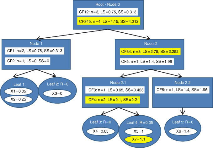
Figure 21.9 Seventh (and last) data value entered: Final form of CF tree.
21.7 Example of BIRCH Clustering, Phase 2: Clustering The Sub-Clusters
Phase 2 often uses agglomerative hierarchical clustering, as we shall perform here. The five CFs CF1, CF2, …, CF5 are the objects that the agglomerative clustering shall be carried out on, not the original data. We use the following simple algorithm:
The cluster centers are as follows:
We start with ![]() . Now, perhaps k = 5 is the optimal cluster solution for this problem. Perhaps not. What we are doing here is forming a set of candidate clustering solutions for k = 5, k = 4, k = 3, and k = 2. We shall then choose the best clustering solution based on a set of evaluative measures. Let us proceed.
. Now, perhaps k = 5 is the optimal cluster solution for this problem. Perhaps not. What we are doing here is forming a set of candidate clustering solutions for k = 5, k = 4, k = 3, and k = 2. We shall then choose the best clustering solution based on a set of evaluative measures. Let us proceed.
The two closest clusters are CF1 and CF3. Combining these CFs, we obtain a new cluster center of ![]() . The remaining cluster centers are
. The remaining cluster centers are
Here, the two nearest clusters are CF4 and CF5. When we combine these CFs, the combined cluster center is ![]() . The remaining cluster centers are
. The remaining cluster centers are
Among these, the two nearest clusters are CF2 and CF1,3. Combining these CFs, we get a new cluster center of ![]() . This leaves us with our last remaining cluster centers:
. This leaves us with our last remaining cluster centers:
Combining these two clusters would result in one big cluster of the entire data set. Each of the above sets of cluster centers represents a candidate clustering solution. We turn now to the problem of how to evaluate these candidate clusters, and so to choose the best clustering solution.
21.8 Evaluating The Candidate Cluster Solutions
In Chapter 23, we will examine methods for measuring cluster goodness. Here we apply one of the methods, the pseudo-F statistic
in order to select the value of k that delivers the optimal clustering solution for our little data set.
For each of the candidate clustering solutions shown above, the pseudo-F statistic and p-value was calculated, and shown in Table 21.1.
Table 21.1 The pseudo-F method selects k = 2 as the preferred clustering solution
| Value of k | MSB | MSE | Pseudo-F | p-Value |
| 2 | 1.1433 | 0.3317 | 17.24 | 0.009 |
| 3 | 0.6533 | 0.0408 | 15.52 | 0.013 |
| 4 | 0.4628 | 0.0289 | 16.02 | 0.024 |
| 5 | 0.3597 | 0.0181 | 19.84 | 0.049 |
The smallest p-value occurs when k = 2. Thus, the preferred clustering solution is for the following cluster centers:
This is indeed the clustering solution preferred by IBM/SPSS Modeler's Two-Step (BIRCH) Algorithm, as the excerpted results in Figure 21.10 indicate, although it should be noted that Modeler uses a different method to select the best model.
Figure 21.10 Modeler's Two-Step (BIRCH) Algorithm selects the same clustering solution that we did.
One may wonder whether we may calculate the pseudo-F statistic, without having recourse to the original data, only the summary statistics in the set of CFs. The answer is, yes, we can, and the proof is left as an exercise.
21.9 Case Study: Applying BIRCH Clustering to The Bank Loans Data Set
Recall the Loans data sets from Chapter 21. The Loans_training data set contains about 150,000 records and the Loans_test data set contains about 50,000 records. The task is to classify loan applications as approved or not (the flag response variable), using the following predictors: debt-to-income ratio, FICO score, and request amount. The amount of interest is included as well, but is a mathematical function of the request amount, and so is perfectly correlated with that predictor.
21.9.1 Case Study Lesson One: Avoid Highly Correlated Inputs to Any Clustering Algorithm
This heading telegraphs our punch line: Analysts should beware of included highly correlated inputs to any clustering algorithm. This section shows just how costly such an error can be.
Define two clustering input collections:
- The With Interest input collection wrongly includes interest as an input, along with the predictors debt-to-income ratio, FICO score, and request amount.
- The No Interest input collection includes only the predictors debt-to-income ratio, FICO score, and request amount as inputs, and does not include interest.
BIRCH clustering was applied to both input collections.5 The With Interest clustering model is shown in Figure 21.11. Two clusters are identified, with a reported mean silhouette (MS) value of about 0.6. The No Interest clustering model is shown in Figure 21.12. Three clusters are identified, with a reported MS value of about 0.4. Thus, the silhouette measure would lead us to believe that the With Interest clustering solution is preferable. However, as we mentioned in Chapter 21, there may be times when the data analyst may have to choose a model that is attuned to the requirements of the client rather than a model that is preferred by a given statistic. Such is the case here.

Figure 21.11 The With Interest clustering model identifies two clusters, and has a higher silhouette value.

Figure 21.12 The No Interest clustering model identifies three clusters.
Figure 21.13 shows how the predictors influenced the composition of the clusters. For the With Interest model, Cluster 1 contains those records

Figure 21.13 Predictor influence on cluster composition. The With Interest model is essentially double counting request amount.
with low FICO score, low request amount (and therefore low interest), and relatively high debt-to-income ratio. Cluster 2 contains records with the opposite levels. Note that the graphs for interest and request amount are essentially identical. This illustrates that we are essentially double counting request amount by including interest, which is a function of request amount, as an input.
The No Interest model, however, shows no such double counting. Let us briefly profile the clusters for the No Interest model.
- Cluster 1: Big Profits, Probably. Cluster 1 contains those with moderately low debt-to-income ratio, moderately high FICO score, and high request amount. The bank would usually like to lend to these people, since they tend to be fairly financially secure. However, they are not as secure as Cluster 3. Most will likely pay back the loan, and the high request amount means that there is plenty of interest (and therefore profit) to be had. But the occasional default will also be high.
- Cluster 2: Iffy Propositions. Cluster 2 consists of applicants with high debt-to-income ratios and low FICO scores. The bank may be advised to tread carefully with this group.
- Cluster 3: Secure Small Profits. Cluster 3 contains the most financially secure applicants, with the lowest debt-to-income ratio and the highest FICO scores. Unfortunately for the bank, these customers are looking for small loans only, that is, the request amount is small. Thus profits will be small, per applicant. But risk is small as well. Approving these customers should, on the whole, be a no-brainer for the bank.
A bank manager may comment that these cluster profiles “feel real,” that is, they seem to reflect actual segments of applicants. Consulting analysts should not underestimate such reality checks.
One way to measure the reality of the clusters is to examine their effects on downstream classification models. So, next we measure the relative efficacy of using cluster membership only (and no other predictors) on a CART model for predicting loan approval. In Chapter 16, we found that the data-driven cost matrix for this problem was as shown in Table 21.2.
Table 21.2 Cost matrix for the bank loan case study
| Predicted Category | |||
| Actual category | |||
Two CART models were trained on the Loans_training data set, using only the cluster membership for the With Interest cluster model and the No Interest cluster model, respectively. These CART models were then evaluated using the Loans_test data set. Table 21.3 shows the contingency table the With Interest model, while Table 21.4 shows the contingency table for the No Interest model.
Table 21.3 Contingency table for With Interest model
| Predicted Category | |||
| Disapprove | Approve | ||
| Actual category | Disapprove | ||
| Approve | |||
Table 21.4 Contingency table for No Interest model
| Predicted Category | |||
| Disapprove | Approve | ||
| Actual category | Disapprove | ||
| Approve | |||
The model costs for these models are as follows:
- With Interest Model:
 , for an average cost of $1306.73 per customer.
 - No Interest Model:
 , for an average cost of $676.98 per customer.
Note that the simple step of being careful to remove the perfectly correlated predictor (interest) from the clustering algorithm has resulted in an estimated increase in decrease in cost of more than $31 million! Of course, the danger of using correlated inputs is not unique to BIRCH clustering; this warning applies across all clustering algorithms.
21.9.2 Case Study Lesson Two: Different Sortings May Lead to Different Numbers of Clusters
Other clustering algorithms require the user to specify a value of k, that is, the number of clusters in the model. However, for BIRCH, the number of clusters is an implicit outcome of the tree-building process. So, the user need not specify k. However, there is a downside. Because of the tree structure inherent in the CF tree, the clustering solution is dependent on the input ordering of the data records. So, different orderings of the data records may lead to different numbers of BIRCH clusters. We illustrate this phenomenon here.
We produced eight different orderings of the approximately 150,000 records in the Loans_training data set. The first ordering was the original ordering of the data used for the No Interest model above. The remaining seven orderings were accomplished as follows:
- Step 1. Generate a sort variable consisting of random draws from a Uniform (0,1) distribution.
- Step 2. Sort the records in ascending order, based on the sort variable.
- Step 3. Run BIRCH on the records obtained in step 2.
The clustering solutions obtained by each of the eight different sort orderings are summarized in Figure 21.14. Note the following:
- Sorts 1, 2, and 8 have k = 3 clusters.
- Sorts 3, 4, 6, and 7 have k = 4 clusters.
- Sort 5 has k = 6 clusters.

Figure 21.14 Pie chart summaries of the BIRCH clusters resulting from the eight different sortings. Which is the best?
When different sortings produce varying values of k, the analyst should try to arrive at a consensus as to the best value of k. At first, we would be tempted to declare k = 4, because it received the most “votes” among the different sortings. For example, the highest MS values are for k = 4 models (see Table 21.5). However, before we declare a winner, it would be helpful to take a closer look at the performance of these cluster models for predicting loan approval.
Table 21.5 Model summaries for BIRCH clusters as classification predictors: eight different data sorts (best performance highlighted)
| TN | FP | FN | TP | Cost Per Customer | k | MS | |
| Sort 1 | 11,360 | 13,584 | 145 | 24,619 | $676.98 | 3 | 0.4 |
| Sort 2 | 16,990 | 7,944 | 5,149 | 19,615 | 3 | 0.4 | |
| Sort 3 | 19,469 | 5,465 | 6,943 | 17,821 | 4 | 0.4 | |
| Sort 4 | 12,444 | 12,490 | 1,437 | 23,327 | $538.48 | 4 | 0.5 |
| Sort 5 | 19,451 | 5,483 | 7,389 | 17,375 | 6 | 0.4 | |
| Sort 6 | 13,538 | 11,396 | 380 | 24,384 | $114.41 | 4 | 0.4 |
| Sort 7 | 11,987 | 12,947 | 121 | 24,643 | $501.96 | 4 | 0.5 |
| Sort 8 | 9,938 | 14,996 | 3 | 24,619 | $1,041.20 | 3 | 0.5 |
For each of the eight sortings, we used the training set to construct a CART model using only the cluster memberships as predictors. We then evaluated each model using the test data set. The somewhat surprising results are shown in Table 21.5 (MS, mean silhouette). The most important column is the “Cost per Customer” column, since these figures affect the bank's bottom line. The three sorts resulting in profit are shown in bold. Note that the three sorts with the highest MS are among the lowest performing models in terms of cost, suggesting that MS may not be a very helpful statistic for our selection of k for this data set.
So, it seems that consensus is eluding us for choice of k with this data set. At this point in the analysis, we are almost beyond the question of choosing k, since the profitability of the models varies considerably for a given value of k. Instead, why not just proceed with the actual clusters obtained with Sort 3 (k = 4) and Sort 5 (k = 6), the two most profitable models? Both of these clustering solutions are remarkably powerful, in that they produce profits using only the cluster memberships as predictors. So the analyst will make a lot of money for the bank if he or she starts with these clusters, and proceeds to enhance these models using the original predictor variables.
In practice, BIRCH is often used to “suggest” a value of k, so that the actual clustering may be performed using some other method, such as k-means clustering. In this case, the analyst may wish to (i) report that BIRCH “suggests” k = 3 through 6, and (ii) proceed with these candidate values of k using k-means or some other clustering algorithm.
Finally, close communication with the client is important at all times, but especially in situations like this. Clients often have a good idea of the types of customers they have, and will often have insight into how many of these groups there are. Further, the client may prefer that the number of clusters be small, in order to facilitate in-company dissemination of the cluster results.
R References
- R Core Team. R: A Language and Environment for Statistical Computing. Vienna, Austria: R Foundation for Statistical Computing; 2012. ISBN: 3-900051-07-0, http://www.R-project.org/. Accessed 2014 Sep 30.
- Charest L, Harrington J, Salibian-Barrera M. 2012. birch: Dealing with very large data sets using BIRCH. R package version 1.2-3. http://CRAN.R-project.org/package=birch.
Exercises
1. Why is BIRCH appropriate for streaming data?
2. Describe the two phases of the BIRCH clustering algorithm.
3. What is a CF?
4. How are the CFs for two clusters merged?
5. Describe the parameters of the CF tree.
6. Why is Phase 2 of the BIRCH algorithm efficient?
7. Why is it bad practice to include two highly correlated inputs to a clustering algorithm?
8. Is the MS value always indicative of the best cluster solution?
Hands-On Exercises
For Exercises 9–12, using the Loans data set, demonstrate that it is bad practice to include interest with the other predictors, as follows:
9. Follow the methodology in Case Study Lesson One to develop cluster models with and without interest.
10. Using the Loans_training data set, develop CART models for predicting loan approval, based on cluster membership only, for the two cluster models.
11. Evaluate each CART model using the Loans_test data set. Provide contingency tables. Compare the model costs, as in Table 21.4.
12. Based on your work in the previous exercises, what is the lesson we should learn?
For Exercises 13–16, using the Loans data set, demonstrate that different sortings may lead to different numbers of clusters. Make sure you do not include interest as an input to the clustering algorithms.
13. Generate four different sortings of the Loans_training data set. Together with the original order from the No Interest model you generated earlier, this makes five different sortings.
14. Run BIRCH on each of the five different sortings. Report the value of k and the MS for each.
15. Calculate model cost for each of the five different sortings. Which model has the highest profitability or the lowest cost?
16. Briefly profile the clusters for the winning model from the previous exercise.