
CHAPTER 9
Markov Processes
In this chapter, we study a class of random processes that possess a certain characteristic that could crudely be described as memoryless. These processes appear in numerous applications including queuing systems, computer communication networks, biological systems, and a wide variety of other applications. As a result of their frequent occurrence, these processes have been studied extensively, and a wealth of theory exists to solve problems related to these processes. We make no attempt to give an exhaustive treatment here, but rather present some of the fundamental concepts involving Markov processes.
9.1 Definition and Examples of Markov Processes
Definition 9.1: A random process, X(t), is said to be a Markov process if for any time instants, t1 ≤ t2 ≤ … ≤ t n ≤ t n+1 the random process satisfies
 (9.1)
(9.1)
To understand this definition, we interpret tn as the present time so that tn + 1 represents some point in the future and t1, t2, …, t n–1 represent various points in the past. The Markovian property then states that given the present, the future is independent of the past. Or, in other words, the future of the random process only depends on where it is now and not on how it got there.
Example 9.1
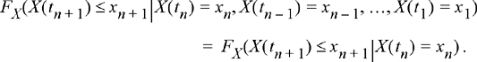
A classical example of a continuous time Markov process is the Poisson counting process studied in the previous chapter. Let X(t) be a Poisson counting process with rate λ. Then its probability mass function satisfies
![]()
Clearly this is independent of {X{tn – 1) = xn– 1,…,X{tx ) = x1]. In fact, the Markovian property must be satisfied because of the independent increments assumption of the Poisson process.
To start with, we will focus our attention on discrete-valued Markov processes in discrete time, better known as Markov chains. Let X[k] be the value of the process at time instant k. Since the process is discrete-valued, X[k] ∈ {X1, x2, x3, …} and we say that if X[k] = xn then the process is in state n at time k. A Markov chain is described statistically by its transition probabilities which are defined as follows.
Definition 9.2: Let X[k] be a Markov chain with states {X1, x2, x3, …}. Then, the probability of transitioning from state i to state j in one time instant is
![]() (9.2)
(9.2)
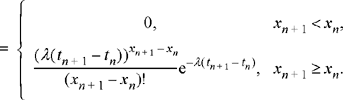
If the Markov chain has a finite number of states, n, then it is convenient to define a transition probability matrix,
 (9.3)
(9.3)
One can encounter processes where the transition probabilities vary with time and therefore need to be explicitly written as a function of k (e.g., pi, j, k ) but we do not consider such processes in this text and henceforth it is assumed that transition probabilities are independent of time.
Example 9.2
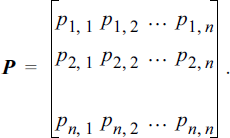
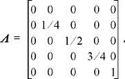
Suppose every time a child buys a kid’s meal at his favorite fast food restaurant he receives one of four superhero action figures. Naturally, the child wants to collect all four action figures and so he regularly eats lunch at this restaurant in order to complete the collection. This process can be described by a Markov chain. In this case, let X[k] ∈ {0,1,2, 3,4} be the number of different action figures that the child has collected after purchasing k meals. Assuming each meal contains one of the four superheroes with equal probability and that the action figure in any meal is independent of what is contained in any previous or future meals, then the transition probability matrix easily works out to be

Initially (before any meals are bought), the process starts in state 0 (the child has no action figures). When the first meal is bought, the Markov chain must move to state 1 since no matter which action figure is contained in the meal, the child will now have one superhero. Therefore, p0, 1 = 1 and p0,j = 0 for all j ≠ 1. If the child has one distinct action figure, when he buys the next meal he has a 25 % chance of receiving a duplicate and a 75% chance of getting a new action figure. Thus, p1,1 = 1/4, p1,2 = 3/4, and p1, j . = 0 for j ≠ 1, 2. Similar logic is used to complete the rest of the matrix. The child might be interested in knowing the average number of lunches he needs to buy until his collection is completed. Or, maybe the child has saved up only enough money to buy 10 lunches and wants to know what are his chances of completing the set before running out of money. We will develop the theory needed to answer such questions.
The transition process of a Markov chain can also be illustrated graphically using a state diagram. Such a diagram is illustrated in Figure 9.1 for the Markov chain in Example 9.2. In the figure, each directed arrow represents a possible transition and the label on each arrow represents the probability of making that transition. Note that for this Markov chain, once we reach state 4, we remain there forever. This type a state is referred to as an absorbing state.
![]()
Figure 9.1 State diagram for the Markov chain of Example 9.2.
Example 9.3 (The Gambler’s Ruin Problem)
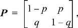
Suppose a gambler plays a certain game of chance (e.g., blackjack) against the “house.” Every time the gambler wins the game, he increases his fortune by one unit (say, a dollar) and every time he loses, his fortune decreases by one unit. Suppose the gambler wins each game with probability p and loses with probability q = I – p. Let Xn represent the amount of the gambler’s fortune after playing the game n times. If the gambler ever reaches the state Xn = 0, the gambler is said to be “ruined” (he has lost all of his money). Assuming that the outcome of each game is independent of all others, the sequence xn, n = 0,1,2, …, forms a Markov chain. The state transition matrix is of the form
The state transition diagram for the gambler’s ruin problem is shown in Figure 9.2a. One might then be interested in determining how long it might take before the gambler is ruined (enters the zero state). Is ruin inevitable for any p, or if the gambler is sufficiently proficient at the game, can he avoid ruin indefinitely? A more realistic alternative to this model is one where the house also has a finite amount of money. Suppose the gambler initially starts with d dollars and the house has b – d dollars so that between the two competitors there is a total of b dollars in the game. Now if the gambler ever gets to the state 0, he is ruined, while if he gets to the state b, he has “broken the bank” (i.e., the house is ruined). Now the Markov chain has two absorbing states as shown in Figure 9.2b. It would seem that sooner or later the gambler must have a run of bad luck sufficient to send him to the 0 state (i.e., ruin) or a run of good luck which will cause him to enter the state b (i.e., break the bank). It would be interesting to find the probabilities of each of these events.

Figure 9.2 State transition diagram for Example 9.3 (The Gamblers Ruin Problem) with (a) one absorbing state and (b) with two absorbing states.
The previous example is one of a class of Markov chains known as random walks. Random walks are often used to describe the motion of a particle. There are many applications that can be described by a random walk that do not involve the movement of a particle, but it is helpful to think of such a particle when describing random walks. In one dimension, a random walk is a Markov chain whose states are the integers and whose transition probabilities satisfy pi, j = 0 for any j ≠ i – 1, i, i + 1. In other words, at each time instant, the state of the Markov chain can either increase by one, stay the same, or decrease by one. If pi, i+ 1 = pi, i– l, then the random walk is said to be symmetric, whereas, if pi, i+ 1 ≠ pi, i –l , the random walk is said to have drift. Often the state space of the random walk will be a finite range of integers, n, n+ 1, n + 2, …,m – l, m (for m > n), in which case the states n and m are said to be boundaries or barriers. The gamblers ruin problem is an example of a random walk with absorbing boundaries, where pn, n = pm, m = 1. Once the particle reaches the boundary, it is absorbed and remains there forever. We could also construct a random walk with reflecting boundaries, in which case pn, n + 1 = pm, m − 1 = 1. That is, whenever the particle reaches the boundary, it is always reflected back to the adjacent state.
Example 9.4 (A Queueing System)
A common example of Markov chains (and Markov processes in general) is that of queueing systems. Consider, for example, a taxi stand at a busy airport. A line of taxis, which for all practical purposes can be taken to be infinitely long, is available to serve travelers. Customers wanting a taxi enter a queue and are given a taxi on a first come, first serve basis. Suppose it takes one unit of time (say, a minute) for the customer at the head of the queue to load himself and his luggage into a taxi. Hence, during each unit of time, one customer in the queue receives service and leaves the queue while some random number of new customers enter the end of the queue. Suppose at each time instant, the number of new customers arriving for service is described by a discrete distribution (p0, pl, p2, …), where pk is the probability of k new customers. For such a system, the transition probability matrix of the Markov chain would look like

The manager of the taxi stand might be interested in knowing the probability distribution of the queue length. If customers have to wait too long, they may get dissatisfied and seek other forms of transportation.
Example 9.5 (A Branching Process)
Branching processes are commonly used in biological studies. Suppose a certain species of organism has a fixed lifespan (one time unit). At the end of its lifespan, the n th organism in the species produces a number of offspring described by some random variable, Yn, whose sample space is the set of non-negative integers. Also, assume that the number of offspring produced by each organism is independent and identically distributed (IID). Then, Xk, the number of species in the organism during the k th generation is a random variable which depends only on the number of organisms in the previous generation. In particular, if ![]() then
then ![]() The transition probability is then
The transition probability is then
![]()
Let HY
(z) be the probability-generating function of the random variable Yn
(i.e., ![]() ). Then, due to the IID nature of the
). Then, due to the IID nature of the ![]() will have a probability-generating function given by [Hy
(z)]i. Hence, the transition probability, pi, j, will be given by the coefficient of zj in the power series expansion of [Hr
(z)]i.
will have a probability-generating function given by [Hy
(z)]i. Hence, the transition probability, pi, j, will be given by the coefficient of zj in the power series expansion of [Hr
(z)]i.
Example 9.6 (A Genetic Model)
Suppose a gene contains n units. Of these units, i are mutant and n – i are normal. Every time a cell doubles, the n units double and each of the two cells receives a gene composed of n units. After doubling, there is a pool of 2n units of which 2i are mutant. These 2n units are grouped into two sets of n units randomly. As we trace a single line of descent, the number of mutant units in each gene forms a Markov chain. Define the k th gene to be in state i (Xk= i) if it is composed of i mutant and n – i normal units. It is not difficult to show that, given Xk = i,
9.2 Calculating Transition and State Probabilities in Markov Chains
The state transition probability matrix of a Markov chain gives the probabilities of transitioning from one state to another in a single time unit. It will be useful to extend this concept to longer time intervals.
Definition 9.3: The n -step transition probability for a Markov chain is
![]() (9.4)
(9.4)
Also, define an n -step transition probability matrix P(n) whose elements are the n -step transition probabilities in Equation (9.4).
Given the one-step transition probabilities, it is straightforward to calculate higher order transition probabilities using the following result.
Theorem 9.1 (Chapman–Kolmogorov Equation):
![]() (9.5)
(9.5)
Proof: First, condition on the event that in the process of transitioning from state i to state j, the Markov chain passes through state k at some intermediate point in time. Then using the principle of total probability
![]() (9.6)
(9.6)
Using the Markov property, the expression reduces to the desired form:
![]() (9.7)
(9.7)
This result can be written in a more compact form using transition probability matrices. It is easily seen that the Chapman–Kolmogorov equations can be written in terms of the n -step transition probability matrices as
![]() (9.8)
(9.8)
Then, starting with the fact that P(1) = P, it follows that P(2) = p(1) p(1) = p2, and using induction, it is established that
![]() (9.9)
(9.9)
Hence, we can find the n -step transition probability matrix through matrix multiplication. If n is large, it may be more convenient to compute Pn via eigendecomposition. In many cases1 the matrix P can be expanded as P = UΛU−1, where Λ is the diagonal matrix of eigenvalues and U is the matrix whose columns are the corresponding eigenvectors. Then,
![]() (9.10)
(9.10)
Another quantity of interest is the probability distribution of the Markov chain at some time instant k. If the initial probability distribution of the Markov chain is known, then the distribution at some later point in time can easily be found. Let πj (k) = Pr(Xk =j) and π(k) be the row vector whose jth element is πj (k). Then
![]() (9.11)
(9.11)
or in vector form,
![]() (9.12)
(9.12)
Example 9.7 (continuation of Example 9.2)
Recall in Example 9.2, the child who purchased kid’s meals at his favorite restaurant in order to collect a set of four superhero action figures. Initially, before any meals are purchased, the child has no action figures and so the initial probability distribution is π(0) = (1,0,0,0,0). Repeated application of Equation (9.12) with the probability transition matrix given in Example 9.2 results in

and so on. It is to be expected that if the child buys enough meals, he will eventually complete the collection (i.e., get to state 4) with probability approaching unity. This can easily be verified analytically by calculating the limiting form of Pk as k → ∞. Recall that for this example, P is a triangular matrix and hence its eigenvalues are simply the diagonal entries. Hence, the diagonal matrix of eigenvalues is
It should be clear that ![]() is a matrix with all zero entries except the one in the lower right corner, which is equal to one. Using MATLAB (or some other math package) to calculate the corresponding matrix of eigenvectors, it is found that
is a matrix with all zero entries except the one in the lower right corner, which is equal to one. Using MATLAB (or some other math package) to calculate the corresponding matrix of eigenvectors, it is found that

Then, using the initial distribution of π(0) = (1,0,0,0,0), the state distribution as X works out to be
![]()
In Example 9.6, it was seen that as k → ∞, the k-step transition probability matrix approached that of a matrix whose rows were all identical. In that case, the limiting product lim k → ∞ π(0)Pk is the same regardless of the initial distribution π(0). Such a Markov chain is said to have a unique steady-state distribution, π. It should be emphasized that not all Markov chains have a steady-state distribution. For example, the Poisson counting process of Example 9.1 clearly does not, since any counting process is a monotonie non-decreasing function of time and, therefore, it is expected that the distribution should skew toward larger values as time progresses.
This concept of a steady-state distribution can be viewed from the perspective of stationarity. Suppose at time k, the process has some distribution, π(k). The distribution at the next time instant is then π(k+ 1) = π(k)P. If π(k) = π(k+ 1), then the process has reached a point where the distribution is stationary (independent of time). This stationary distribution, π, must satisfy the relationship
![]() (9.13)
(9.13)
In other words, π (if it exists) is the left eigenvector of the transition probability matrix P, that corresponds to the eigenvalue λ = 1. The next example shows that this eigenvector is not always unique.
Example 9.8 (The Gambler’s Ruin revisited)
Suppose a certain gambler has $5 and plays against another player (the house). The gambler decides that he will play until he either doubles his money or loses it all. Suppose the house has designed this game of chance so that the gambler will win with probability p = 0.45 and the house will win with probability q = 0.55. Let Xk be the amount of money the gambler has after playing the game k times. The transition probability matrix for this Markov chain is

This matrix has (two) repeated eigenvalues of λ = 1, and the corresponding eigenvectors are [10 0 0 0 0 0 0 0 0 0] and [00 0 0 0 0 0 0 0 0 l] Note that any linear combination of these will also be an eigenvector. Therefore, any vector of the form [p00000000l–p] is a left eigenvector off and hence there is no unique stationary distribution for this Markov chain. For this example, the limiting form of the state distribution of the Markov chain depends on the initial distribution. The limiting form of Pk can easily be found to be

Using the initial distribution π(0) = [0 000010000 0] (that is, the gambler starts off in state 5), then it is seen that the steady-state distribution is ![]() . So, when the gambler starts with $5, he has about a 73% chance of losing all of his money and about a 27% chance of doubling his money.
. So, when the gambler starts with $5, he has about a 73% chance of losing all of his money and about a 27% chance of doubling his money.
As seen in Example 9.7, with some Markov chains, the limiting form of P k (as k → ∞) does not necessarily converge to a matrix whose rows are all identical. In that case, the limiting form of the state distribution will depend on the starting distribution. In the case of the gambler’s ruin problem, we probably could have guessed this behavior. If the gambler had started with very little money, we would expect him to end up in the state of ruin with very high probability; whereas, if the gambler was very wealthy and the house had very little money, we would expect a much greater chance of the gambler eventually breaking the house. Accordingly, our intuition tells us that the probability distribution of the gamblers ultimate state should depend on the starting state.
In general, there are several different manners in which a Markov chain’s state distribution can behave as k → ∞ In some cases, ![]() does not exist. Such would be the case when the process tends to oscillate between two or more states. A second possibility, as in Example 9.7, is that
does not exist. Such would be the case when the process tends to oscillate between two or more states. A second possibility, as in Example 9.7, is that ![]() does in fact converge to a fixed distribution, but the form of this limiting distribution depends on the starting distribution. The last case is when,
does in fact converge to a fixed distribution, but the form of this limiting distribution depends on the starting distribution. The last case is when, ![]() That is the state distribution converges to some fixed distribution, π, and the form of π is independent of the starting distribution. Here, the transition probability matrix, P, will have a single (not repeated) eigenvalue at λ = 1, and the corresponding eigenvector (properly normalized) will be the steady-state distribution, π. Furthermore, the limiting form of Pk
will be one whose rows are all identical and equal to the steady-state distribution, π. In the next section, we look at some conditions that must be satisfied for the Markov chain to achieve a unique steady-state distribution.
That is the state distribution converges to some fixed distribution, π, and the form of π is independent of the starting distribution. Here, the transition probability matrix, P, will have a single (not repeated) eigenvalue at λ = 1, and the corresponding eigenvector (properly normalized) will be the steady-state distribution, π. Furthermore, the limiting form of Pk
will be one whose rows are all identical and equal to the steady-state distribution, π. In the next section, we look at some conditions that must be satisfied for the Markov chain to achieve a unique steady-state distribution.
Example 9.9
 In this example, we provide the MATLAB code to simulate the distribution of the queue length of the taxi stand described in Example 9.4. For this example, we take the number of arrivals per time unit, X, to be a Poisson random variable whose PMF is
![]()
Recall that in the taxi stand, one customer is served per time unit (assuming there is a least one customer in the queue waiting to be served). The following code can be used to estimate and plot the PMF of the queue length. The average queue length was also calculated to be 3.36 customers for an arrival rate of λ = 0.85 customers per time unit. Figure 9.3 shows a histogram of the PMF of the queue length for the same arrival rate.

Figure 9.3 Histogram of the queue length for the taxi stand of Example 9.4 assuming a Poisson arrival process with an average arrival rate of 0.85 arrivals per time unit.


9.3 Characterization of Markov Chains
Using the methods presented in the previous sections, calculating the steady-state distribution of a Markov chain requires performing an eigendecomposition of the transition probability matrix, P. If the number of states in the Markov chain is large (or infinite), performing the required linear algebra may be difficult (or impossible). Thus, it would be useful to seek alternative methods to determine if a steady-state distribution exists, and if so, to calculate it. To develop the necessary theory, we must first proceed through a sequence of definitions and classifications of the states of a Markov chain.
Definition 9.4: State j is accessible from state i if for some finite ![]() This simply means that if the process is in state i, it is possible for the process to get to state j in a finite amount of time. Furthermore, if state j is accessible from state i and state i is accessible from state j, then the states i and j are said to communicate. It is common to use the shorthand notation i ↔ j to represent the relationship “state i communicates with state j.”
This simply means that if the process is in state i, it is possible for the process to get to state j in a finite amount of time. Furthermore, if state j is accessible from state i and state i is accessible from state j, then the states i and j are said to communicate. It is common to use the shorthand notation i ↔ j to represent the relationship “state i communicates with state j.”
The states of any Markov chain can be divided into sets or classes of states where all the states in a given class communicate with each other. It is possible for the process to move from one communicating class of states to another, but once that transition is made, the process can never return to the original class. If it did, the two classes would communicate with each other and hence would be a part of a single class.
Definition 9.5: A Markov chain for which all of the states are part of a single communicating class is called an irreducible Markov chain. Also, the corresponding transition probability matrix is called an irreducible matrix.
The examples in Section 9.1 can be used to help illustrate these concepts. For both processes in Examples 9.1 and 9.2, none of the states communicate with any other states. This is a result of the fact that both processes are counting processes and as a result, it is impossible to go backward in the chain of states. Therefore, if j > i, state j is accessible from state i but state i is not accessible from state j. As a result, for any counting process, all states form a communication class of their own. That is, the number of classes is identical to the number of states. In the gambler’s ruin problem of Example 9.3, the two absorbing states do not communicate with any other state since it is impossible to ever leave an absorbing state, while all the states in between communicate with each other. Therefore, this Markov chain has three communicating classes; the two absorbing states each form of class to themselves, while the third class consists of all the states in between.
The queueing system (taxi stand) of Example 9.4 represents a Markov chain where all states communicate with each other, and therefore that Markov chain is irreducible. For the branching process of Example 9.5, all states communicate with each other except the state 0, which represents the extinction of the species, which presumably is an absorbing state. The genetic model of Example 9.6 is similar to the gambler’s ruin problem in that the Markov chain has two absorbing states at the end points, while everything in between forms a single communicating class.
Definition 9.6: The period of state i, d(i), is the greatest common divisor of all integers n ≥ 1 such that ![]() . Stated another way, d(i) is the period of state i if any transition from state i to itself must occur in a number of steps that is a multiple of d (i). Furthermore, a Markov chain for which all states have a period of d (i) = 1 is called an aperiodic Markov chain.
. Stated another way, d(i) is the period of state i if any transition from state i to itself must occur in a number of steps that is a multiple of d (i). Furthermore, a Markov chain for which all states have a period of d (i) = 1 is called an aperiodic Markov chain.
Most Markov chains are aperiodic. The class of random walks is an exception. Suppose a Markov chain defined on the set of integers has transition probabilities that satisfy
 (9.14)
Then each state will have a period of 2. If we add absorbing boundaries to the random walk, then the absorbing states are not periodic because for the absorbing states, ![]() for all n and thus the period of an absorbing state is 1. It is left as an exercise for the reader (see Exercise 9.26) to establish the fact that the period is a property of a class of communicating states. That is, if i ↔ j, then d (i) = d (j) and therefore all states in the same class must have the same period.
for all n and thus the period of an absorbing state is 1. It is left as an exercise for the reader (see Exercise 9.26) to establish the fact that the period is a property of a class of communicating states. That is, if i ↔ j, then d (i) = d (j) and therefore all states in the same class must have the same period.
Definition 9.7: Let ![]() be the probability that given a process is in state i, the first return to state i will occur in exactly n steps. Mathematically,
be the probability that given a process is in state i, the first return to state i will occur in exactly n steps. Mathematically,
![]() (9.15)
(9.15)
Also, define fi, i to be the probability that the process will eventually return to state i. The probability of eventual return is related to the first return probabilities by
![]() (9.16)
(9.16)
It should be noted that the first return probability ![]() is not the same thing as the n-step transition probability, but the two quantities are related. To develop this relationship, it is observed that
is not the same thing as the n-step transition probability, but the two quantities are related. To develop this relationship, it is observed that
 (9.17)
In Equation (9.17), ![]() is taken to be equal to 1 and
is taken to be equal to 1 and ![]() is taken to be equal to 0. Given the n-step transition probabilities, p(n)
ii
, one could solve the preceding system of equations for the first return probabilities. However, since the previous equation is a convolution, this set of equations may be easier to solve using frequency domain techniques. Define the generating functions1,
is taken to be equal to 0. Given the n-step transition probabilities, p(n)
ii
, one could solve the preceding system of equations for the first return probabilities. However, since the previous equation is a convolution, this set of equations may be easier to solve using frequency domain techniques. Define the generating functions1,
![]() (9.18)
(9.18)
![]() (9.19)
(9.19)
It is left as an exercise for the reader (see Exercise 9.27) to demonstrate that these two generating functions are related by
![]() (9.20)
(9.20)
This relationship provides an easy way to compute the first return probabilities from the n-step transition probabilities. Note that if the transition probability matrix is known, then calculating the generating function, Pi, i
(z), is straightforward. Recall that ![]() and therefore if [U]i,j is the element in the ith row and jth column of U, then
and therefore if [U]i,j is the element in the ith row and jth column of U, then
 (9.21)
Forming the generating function from this equation results in
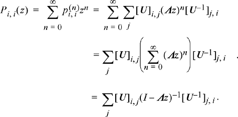 (9.22)
In other words, Pi, i
(z) is the element in the ith row and ith column of the matrix ![]()
Definition 9.8: The i th state of a Markov chain is transient if fi, i > 1 and recurrent if fi, i = 1. Since fi represents the probability of the process eventually returning to state i given that it is in state i, the state is transient if there is some non-zero probability that it will never return, and the state is recurrent if the process must eventually return with probability 1.
Theorem 9.2: State i of a Markov chain is recurrent if and only if
![]() (9.23)
(9.23)
Since this sum represents the expected number of returns to state i, it follows that a state is recurrent if and only if the expected number of returns is infinite.
Proof: First, note that ![]() . From Equation (9.20), this would imply that
. From Equation (9.20), this would imply that
![]() (9.24)
(9.24)
![]() (9.25)
(9.25)
If state i is transient, then fi,i
≤ 1 and hence, ![]() , whereas if state i is recurrent, fi,i = 1 and
, whereas if state i is recurrent, fi,i = 1 and ![]() .
.
We leave it to the reader (see Exercise 9.29) to verify that recurrence is a class property. That is, if one state in a communicating class is recurrent, then all are recurrent, and if one is transient, then all are transient.
Example 9.10
Consider a random walk on the integers (both positive and negative) that initially starts at the origin (X0 = 0). At each time instant, the process either increases by 1 with probability p or decreases by 1 with probability 1 – p:

First note that this Markov chain is periodic with period 2 and hence ![]() for any odd n. For even n, given the process is in state i, the process will be in state i again n time instants later if during those time instants the process increases n/2 times and decreases n/2 times. This probability follows a binomial distribution so that
for any odd n. For even n, given the process is in state i, the process will be in state i again n time instants later if during those time instants the process increases n/2 times and decreases n/2 times. This probability follows a binomial distribution so that
![]()
To determine if the states of this random walk are recurrent or transient, we must determine whether or not the series
![]()
converges. To help make this determination, the identity
![]()
is used. This identity can easily be verified by expanding the binomial on the right hand side in powers of X and confirming (after a little algebra) that the coefficients of the power series expansion do take on the desired form. Applying this identity results in
![]()
Note that for a probability p, 4p(l – p)≤ 1 with equality if and only if p = 1/2. Therefore, the series converges and all states are transient if p ≠ 1/2, while if p = 1/2, the series diverges and all states are recurrent.
Definition 9.9: The mean time to first return for a recurrent state i of a Markov chain is
![]() (9.26)
(9.26)
If the state is transient, then the mean time to first return must be infinite, since with some non-zero probability, the process will never return.
Definition 9.10: A recurrent state is referred to as null recurrent if μi = ∞, while the state is positive recurrent if μi ≤ ∞.
The mean time to first return of a recurrent state is related to the steady-state probability of the process being in that state. To see this, define a sequence of random variables T1, T2, T3, … where Tm represents the time between the m − 1 th and mth returns to the state i. That is, suppose that Xk = i for some time instant k which is sufficiently large so that the process has pretty much reached steady state. The process then returns to state i at time instants k + T1, k+ τ1 + T2, k+ τ1 + T2 + T3, and so on. Over some period of time where the process visits state i exactly n times, the fraction of time the process spends in state i can be written as
 (9.27)
As n → ∞ (assuming the process is ergodic), the left hand side of the previous equation becomes the steady-state probability that the process is in state i, πi . Furthermore, due to the law of large numbers, the denominator of the right hand side converges to μi This proves the following key result.
Theorem 9.3: For an irreducible, aperiodic, recurrent Markov chain, the steady-state distribution is unique and is given by
![]() (9.28)
(9.28)
Note that if a state is positive recurrent, then πi > 0, while if a state is null recurrent, then πi= 0. Note that for any transient state, μi = ∞ and as a result, πi = 0.
Example 9.11
Continuing with the random walk from the previous example, the generating function for the n-step transition probabilities is found to be
![]()
Using the relationship Pi,i(z) − 1 = Pi i {z)Fi,i(z), the generating function for the first return probabilities is
![]()
Since the random walk is only recurrent for ρ = 1/2, we consider only that case so that ![]() The mean time to first return can be found directly from the generating function.
The mean time to first return can be found directly from the generating function.
![]()
Thus, when the transition probabilities of the random walk are balanced so that all states are recurrent, then the mean time to first return is infinite and, in fact, all states are null recurrent.
9.4 Continuous Time Markov Processes
In this section, we investigate Markov processes where the time variable is continuous. In particular, most of our attention will be devoted to the so-called birth–death processes which are a generalization of the Poisson counting process studied in the previous chapter. To start with, consider a random process X(t) whose state space is either finite or countably infinite so that we can represent the states of the process by the set of integers,
X(t) ∈ {…,–3,–2,–1,0, 1,2,3, …}. Any process of this sort that is a Markov process has the interesting property that the time between any change of states is an exponential random variable. To see this, define Ti to be the time between the ith and the i + 1 th change of state and let hi (t) be the complement to its CDF, hi (t) = Pr(T i > t). Then, for t > 0, s > 0
![]() (9.29)
(9.29)
Due to the Markovian nature of the process, Pr(Ti > t + s | Ti > s) = Pr(Ti > t) and hence the previous equation simplifies to
![]() (9.30)
(9.30)
The only function which satisfies this type of relationship for arbitrary t and s is an exponential function of the form ![]() for some constant pi
. Furthermore, for this function to be a valid probability, the constant pi
must not be negative. From this, the PDF of the time between change of states is easily found to be
for some constant pi
. Furthermore, for this function to be a valid probability, the constant pi
must not be negative. From this, the PDF of the time between change of states is easily found to be ![]()
As with discrete-time Markov chains, the continuous-time Markov process can be described by its transition probabilities.
Definition 9.11: Define pt, j (t) = Pr(X(to + t) = j|X(to) = i) to be the transition probability for a continuous time Markov process. If this probability does not depend on to, then the process is said to be a homogeneous Markov process.
Unless otherwise stated, we assume for the rest of this chapter that all continuous time Markov processes are homogeneous. The transition probabilities, pi, j (t), are somewhat analogous to the n-step transition probabilities used in the study of discrete-time processes and as a result, these probabilities satisfy a continuous time version of the Chapman–Kolmogorov equations:
![]() (9.31)
(9.31)
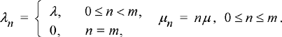
One of the most commonly studied class of continuous time Markov processes is the birth–death process. These processes get their name from applications in the study of biological systems, but they are also commonly used in the study of queueing theory, and many other applications. The birth–death process is similar to the discrete-time random walk studied in the previous section in that when the process changes states, it either increases by 1 or decreases by 1. As with the Poisson counting process, the general class of birth–death processes can be described by the transition probabilities over an infinitesimal period of time, Δt. For a birth–death process,
 (9.32)
The parameter λi is called the birth rate while μi is the death rate when the process is in state i. In the context of queueing theory, λi and μi are referred to as the arrival and departure rates, respectively.
Similar to what was done with the Poisson counting process, by letting s = Δt in Equation (9.31) and then applying the infinitesimal transition probabilities, a set of differential equations can be developed that will allow us to solve for the general transition probabilities. From Equation (9.31),
 (9.33)
Rearranging terms and dividing by Δt produces
![]() (9.34)
(9.34)
Finally, passing to the limit as Δt → 0 results in
![]() (9.35)
(9.35)
This set of equations is referred to as the forward Kolmogorov equations. One can follow a similar procedure (see Exercise 9.32) to develop a slightly different set of equations known as the backward Kolmogorov equations,
![]() (9.36)
(9.36)
For all but the simplest examples, it is very difficult to find a closed-form solution for this system of equations. However, the Kolmogorov equations can lend some insight into the behavior of the system. For example, consider the steady-state distribution of the Markov process. If a steady state exists, we would expect that as ![]() independent of i and also that
independent of i and also that ![]() Plugging these simplifications into the forward Kolmogorov equations leads to
Plugging these simplifications into the forward Kolmogorov equations leads to
![]() (9.37)
(9.37)
These equations are known as the global balance equations. From them, the steady-state distribution can be found (if it exists). The solution to the balance equations is surprisingly easy to obtain. First, we rewrite the difference equation in the more symmetric form
![]() (9.38)
(9.38)
Next, assume that the Markov process is defined on the states j = 0,1,2,…. Then the previous equation must be adjusted for the end point j = 0 according to (assuming μ0 = 0 which merely states that there can be no deaths when the population size is zero)
![]() (9.39)
(9.39)
Combining Equations (9.38) and (9.39) results in
![]()
which leads to the simple recursion
 (9.41)
whose solution is given by
 (9.42)
This gives the πj in terms of π0. In order to determine π0, the constraint that the πj must form a distribution is imposed.
 (9.43)
This completes the proof of the following theorem.
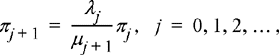
Theorem 9.4: For a Markov birth–death process with birth rate λn, n = 0,1,2, …, and death rate μn , n = 1,2, 3, …, the steady-state distribution is given by
 (9.44)
If the series in the denominator diverges, then πk =0 for any finite k. This indicates that a steady-state distribution does not exist. Likewise, if the series converges, the will be non-zero resulting in a well-behaved steady-state distribution.
Example 9.12 (The M/M/1 Queue)
In this example, we consider the birth–death process with constant birth rate and constant death rate. In particular, we take
![]()
This model is commonly used in the study of queueing systems and, in that context, is referred to as the M/M/1 queue. In this nomenclature, the first “M” refers to the arrival process as being Markovian, the second “M” refers to the departure process as being Markovian, and the “1” is the number of servers. So this is a single server queue, where the interarrival time of new customers is an exponential random variable with mean 1/λ and the service time for each customer is exponential with mean 1/μ. For the M/M/1 queueing system, λi– 1 /μi = λ/ μ for all i so that
![]()
The resulting steady-state distribution of the queue size is then

Hence, if the arrival rate is less than the departure rate, the queue size will have a steady state. It makes sense that if the arrival rate is greater than the departure rate, then the queue size will tend to grow without bound.
Example 9.13 (The M/M/co Queue)
Next suppose the last example is modified so that there are an infinite number of servers available to simultaneously provide service to all customers in the system. In that case, there are no customers ever waiting in line, and the process X{t) now counts the number of customers in the system (receiving service) at time t. As before, we take the arrival rate to be constant λn = λ, but now the departure rate needs to be proportional to the number of customers in service, μn = nμ. In this case, λ1–1/μi = λ/{iμ) and
![]()
Note that the series converges for any λ and μ, and hence the M/M/∞ queue will always have a steady-state distribution given by
![]()
Example 9.14
This example demonstrates one way to simulate the M/M/1 queueing system of Example 9.12. One realization of this process as produced by the code that follows is illustrated in Figure 9.4. In generating the figure, we use an average arrival rate of λ = 20 customers per hour and an average service time of 1
/μ = 2 minutes. This leads to the condition λ≤μ and the M/M/1 queue exhibits stable behavior. The reader is encouraged to run the program for the case when λ>μ to observe the unstable behavior (the queue size will tend to grow continuously over time).

Figure 9.4 Simulated realization of the birth/death process for an M/M/1 queueing system of Example 9.12.


If the birth–death process is truly modeling the size of a population of some organism, then it would be reasonable to consider the case when λQ = 0. That is, when the population size reaches zero, no further births can occur. In that case, the species is extinct and the state X(t) = 0 is an absorbing state. A fundamental question would then be, is extinction a certain event and if not what is the probability of the process being absorbed into the state of extinction? Naturally, the answer to these questions would depend on the starting population size. Let qt be the probability that the process eventually enters the absorbing state, given that it is initially in state i. Note that if the process is currently in state i, after the next transition, the birth–death process must be either in state i – 1 or state i + 1. The time to the next birth, Bi , is a random variable with an exponential distribution with a mean of 1/λi , while the time to the next death is an exponential random variable, D i , with a mean of 1/μi . Thus, the process will transition to state i + 1 if Bi ≤ Di , otherwise it will transition to state i – 1. The reader can easily verify that Pr(Bi ≤ D i ) = λi/(λj + μi ). The absorption probability can then be written as
 (9.45)
This provides a recursive set of equations that can be solved to find the absorption probabilities. To solve this set of equations, we rewrite them as
![]() (9.46)
(9.46)
After applying this recursion repeatedly and using the fact that q0 = 1,
 (9.47)
Summing this equation from i = 1, 2, …, n results in
 (9.48)
Next, suppose that the series on the right hand side of the previous equation diverges as n → ∞. Since the qi are probabilities, the left hand side of the equation must be bounded, which implies that q1 = 1. Then from Equation (9.47), it is determined that qn must be equal to 1 for all n. That is, if
 (9.49)
then absorption will eventually occur with probability 1 regardless of the starting state. If q1 ≤ 1 (absorption is not certain), then the preceding series must converge to a finite number.
It is expected in that case that as n → ∞, qn → 0. Passing to the limit as n → ∞ in Equation (9.48) then allows a solution for ql of the form
 (9.50)
Furthermore, the general solution for the absorption probability is
 (9.51)
Example 9.15
Consider a population model where both the birth and death rates are proportional to the population, λn = nλ, μn = nμ. For this model,
![]()
Therefore, if λ≤μ, the series diverges and the species will eventually reach extinction with probability 1. if λ > μ,
![]()
and the absorption (extinction) probabilities are
![]()
Continuous time Markov processes do not necessarily need to have a discrete amplitude as in the previous examples. In the following, we discuss a class of continuous time, continuous amplitude Markov processes. To start with, it is noted that for any time instants t0 ≤tl≤t2, the conditional PDF of a Markov process must satisfy the Chapman–Kolmogorov equation
![]() (9.52)
(9.52)
This is just the continuous amplitude version of Equation (9.31). Here, we use the notation f(x2, t2 |x1, t1) to represent the conditional probability density of the process X(t2) at the point x2 conditioned on X(t1) = X1. Next, suppose we interpret these time instants as t0 = 0, t1 = t, and t2 = t+ Δt. In this case, we interpret x2 – x1 = Δx as the the infinitesimal change in the process that occurs during the infinitesimal time instant Δt and f(x2, t2 |x1, t1) is the PDF of that increment.
Define ΦΔx (ω) to be the characteristic function of Δx = x2 – x1:
![]() (9.53)
(9.53)
We note that the characteristic function can be expressed in a Taylor series as
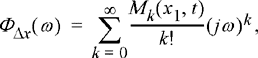 (9.54)
where Mk (x1, t) = E[(x2 –x1)k|(x1, t)] is the kth moment of the increment Δx. Taking inverse transforms of this expression, the conditional PDF can be expressed as
 (9.55)
Inserting this result into the Chapman–Kolmogorov equation, Equation (9.52), results in
 (9.56)
Subtracting f(x2, t|x0, t0) from both sides of this equation and dividing by Δt results in
 (9.57)
Finally, passing to the limit as Δt → 0 results in the partial differential equation
 (9.58)
where the function Kk (x, t) is defined as
![]() (9.59)
(9.59)
For many processes of interest, the PDF of an infinitesimal increment can be accurately approximated from its first few moments and hence we take Kk (x, t) = 0 for k > 2. For such processes, the PDF must satisfy
 (9.60)
This is known as the (one-dimensional) Fokker–Planck equation and is used extensively in diffusion theory to model the dispersion of fumes, smoke, and similar phenomenon.
In general, the Fokker–Planck equation is notoriously difficult to solve and doing such is well beyond the scope of this text. Instead, we consider a simple special case where the functions K1(x, t) and K2 (x, t) are constants, in which case the Fokker–Planck equation reduces to
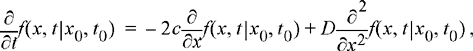 (9.61)
where in diffusion theory, D is known as the coefficient of diffusion and c is the drift. This equation is used in models that involve the diffusion of smoke or other pollutants in the atmosphere, the diffusion of electrons in a conductive medium, the diffusion of liquid pollutants in water and soil, and the difussion of plasmas. This equation can be solved in several ways. Perhaps one of the easiest methods is to use Fourier transforms. This is explored further in the exercises where the reader is asked to show that (taking x0 = 0 and t0 = 0) the solution to this diffusion equation is
 (9.62)
That is, the PDF is Gaussian with a mean and variance which changes linearly with time. For the case when c = 0, this is the Wiener process discussed in Section 8.5. The behavior of this process is explored in the next example.
Example 9.16
In this example, we model the diffusion of smoke from a forest fire that starts in a National Park at time t = 0 and location X = 0. The smoke from the fire drifts in the positive X directioin due to wind blowing at 10 miles per hour, and the diffusion coefficient is 1 square mile per hour. The probability density function is given in Equation (9.62). We provide a three-dimensional rendition of this function in Figure 9.5 using the following MATLAB program.

Figure 9.5 Observations of the PDF at different time instants showing the drift and dispersion of smoke for Example 9.16.


9.5 Engineering Application: A Computer Communication Network
Consider a local area computer network where a cluster of nodes are connected by a common communication line. Suppose for simplicity that these nodes occasionally need to transmit a message of some fixed length (referred to as a packet). Also, assume that the nodes are synchronized so that time is divided into slots, each of which is sufficiently long to support one packet. In this example, we consider a random access protocol known as slotted Aloha. Messages (packets) are assumed to arrive at each node according to a Poisson process. Assuming there are a total of n nodes, the packet arrival rate at each node is assumed to be λ/n so that the total arrival rate of packets is fixed at λ packets/slot. In slotted Aloha, every time a new packet arrives at a node, that node attempts to transmit that packet during the next slot. During each slot, one of three events can occur:(1) no node attempts to transmit a packet, in which case the slot is said to be idle; (2) exactly one node attempts to transmit a packet, in which case the transmission is successful; (3) more than one node attempts to transmit a packet, in which case a collision is said to have occurred. All nodes involved in a collision will need to retransmit their packets, but if they all retransmit during the next slot, then they will continue to collide and the packets will never be successfully transmitted. All nodes involved in a collision are said to be backlogged until their packet is successfully transmitted. In the slotted Aloha protocol, each backlogged node chooses to transmit during the next slot with probability p (and hence chooses not to transmit during the next slot with probability 1 – p). Viewed in an alternative manner, every time a collision occurs, each node involved waits a random amount of time until they attempt retransmission, where that random time follows a geometric distribution.
This computer network can be described by a Markov chain, Xk = number of backlogged nodes at the end of the k th slot. To start with, we evaluate the transition probabilities of the Markov chain, pi, j . Assuming that there are an infinite number of nodes (or a finite number of nodes each of which could store an arbitrary number of backlogged packets in a buffer), we note that
![]() (9.63)
(9.63)
![]() (9.64)
(9.64)
Using these equations, it is straightforward to determine that the transition probabilities are given by
 (9.65)
In order to get a feeling for the steady-state behavior of this Markov chain, we define the drift of the chain in state i as
![]() (9.66)
(9.66)
Given that the chain is in state i, if the drift is positive, then the number of backlogged nodes will tend to increase; whereas, if the drift is negative, the number of backlogged nodes will tend to decrease. Crudely speaking, a drift of zero represents some sort of equilibrium for the Markov chain. Given the preceding transition probabilities, the drift works out to be
![]() (9.67)
(9.67)
Assuming that p « 1, then we can use the approximations (1 − p) ≈ d1 and (1 − p)i ≈ e−ip to simplify the expression for the drift,
![]() (9.68)
(9.68)
The parameter g(i) has the physilcal interpretation of the average number of transmissions per slot given there are i backlogged states. To understand the significance of this result, the two terms in the expression for the drift are plotted in Figure 9.6. The first term, λ, has the interpretation of the average number of new arrivals per slot, while the second term, g exp (−g), is the average number of successful transmissions per slot or the average departure rate. For a very small number of backlogged states, the arrival rate is greater than the departure rate and the number of backlogged states tends to increase. For moderate values of i, the departure rate is greater than the arrival rate and the number of backlogged states tends to decrease. Hence, the drift of the Markov chain is such that the system tends to stabilize around the point marked stable equilibrium in Figure 9.6. This is the first point where the two curves cross. Note, however, that for very large i, the drift becomes positive again. If the number of backlogged states ever becomes large enough to push the system to the right of the point marked unstable equilibrium in the figure, then the number of backlogged nodes will tend to grow without bound and the system will become unstabe.

Figure 9.6 Arrival rate and successful transmission rate for a slotted Aloha system.
Note that the value of λ represents the throughput of the system. If we try to use a value of λ which is greater than the peak value of g exp (−g), then the drift will always be positive and the system will be unstable from the beginning. This maximum throughput occurs when g(i) = 1 and has a value of λmax = 1/e. By choosing an arrival rate less than λmax, we can get the system to operate near the stable equilibrium, but sooner or later, we will get a string of bad luck and the system will drift into the unstable region. The lower the arrival rate, the longer it will take (on average) for the system to become unstable, but at any arrival rate, the system will eventually reach the unstable region. Thus, slotted Aloha is inherently an unstable protocol. As a result, various modifications have been proposed which exhibit stable behavior.
9.6 Engineering Application: A Telephone Exchange
Consider a base station in a cellular phone system. Suppose calls arrive at the base station according to a Poisson process with some arrival rate λ. These calls are initiated by mobile units within the cell served by that base station. Furthermore, suppose each call has a duration that is an exponential random variable with some mean, 1/μ. The base station has some fixed number of channels, m, that can be used to service the demands of the mobiles in its cell. If all m channels are being used, any new call that is initiated cannot be served and the call is said to be blocked. We are interested in calculating the probability that when a mobile initiates a call, the customer is blocked.
Since the arrival process is memoryless and the departure process is memoryless, the number of calls being serviced by the base station at time t, X(t), is a birth−death Markov process. Here, the arrival rate and departure rates (given there are n channels currently being used) are given by
 (9.69)
The steady-state distribution of this Markov process is given by Equation (9.44). For this example, the distribution is found to be
 (9.70)
The blocking probability is just the probability that when a call is initiated, it finds the system in state m. In steady state, this is given by πm and the resulting blocking probability is the so-called Erlang-B formula,
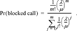 (9.71)
This equation is plotted in Figure 9.7 for several values of m. The horizontal axis is the ratio of λ/ μ which is referred to in the telephony literature as the traffic intensity. As an example of the use of this equation, suppose a certain base station had 60 channels available to service incoming calls. Furthermore, suppose each user initiated calls at a rate of 1 call per 3 hours and calls had an average duration of 3 minutes (0.05 hours). If a 2% probability of blocking is desired, then from Figure 9.7 we determine that the system can handle a traffic intensity of approximately 50 Erlangs. Note that each user generates an intensity of
![]() (9.72)
(9.72)
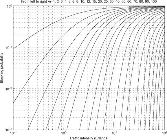
Figure 9.7 The Erlang-B formula.
Hence, a total of 50*60 = 3000 mobile users per cell could be supported while still maintaining a 2% blocking probability.
Exercises
Section 9.1: Definition and Examples of Markov Processes
9.1 For a Markov chain, prove or disprove the following statement:
![]()
9.2 A Diffusion Model - Model the diffusion of electrons and holes across a potential barrier in an electronic device as follows. We have n black balls (electrons) in urn A and n whiteballs (holes) in urn B. An experimental outcome selects randomly one ball from each urn. The ball from urn A is placed in urn B and that from urn B is placed in A. Let the state of the process be the number of black balls in urn A. (By knowing the number of black balls in urn A, we know the composition of both urns.) Let k denote the state of the process. Find the transition probabilities, pi, j .
9.3 Let X[n] be the sum of n independent rolls of a fair (cubicle) die.
(b) Define a new process according to Y[n] = X[n] mod 3. That is, Y[n] ∈ {0, 1, 2} is related to X[n] by X[n] = 3q + Y[n] for a non-negative integer q. Find the transition probability matrix for the process Y[n].
(c) Now suppose Z[n] = X[n] mod 5. Find the transition matrix for Z[n].
9.4 Suppose we label the spaces on a monopoly board as {0, 1, 2, …, 39} where,
0 = Go,
1 = Mediterranean Ave.,
2 = Community Chest,
3 = Baltic Ave.,
…
39 = Boardwalk.
Let X[k] be the location of a player after k turns. On each turn, a player moves by rolling two (six-sided) dice and moving forward the number of places indicated by the sum of the two dice. Any time the roll of the dice causes the player to land on space 30 (Go to Jail) the player’s token is immediately moved to space 10 (Jail). Describe the elements of the transition probability matrix, pi, j
, for the monopoly Markov chain X[k].
9.5 N balls labeled 1 through N are placed in Box 1 while a Box 2 is initially empty. At each time instant, one of the N balls is chosen (with equally probability) and moved to the other box. Let X[k] be the number of balls in Box 1 at time instant k. Draw a state diagram and find the transition probability matrix for this Markov chain. Note: This is known as the Ehrenfest chain and was developed by the dutch Physicist Paul Ehrenfest for the study of molecular dynamics.
9.6 An Inventory Model — A hot dog vendor operates a stand where the number of hot dogs he sells each day is modeled as a Poisson random variable with a mean value of 100. Let X[k] represent the number of hot dogs the vendor has at the beginning of each day. At the end of the day, if his inventory of hot dogs on hand falls below some minimum value, α, then the vendor goes out that evening and purchses enough hot dogs to bring the total of his inventory to β. Write an equation to describe the elements of the transition probability matrix, pi, j ., for this inventory process.
9.7 A Web Search Engine Model - Suppose after we enter some keywords into our web search engine it finds five pages that contain those keywords. We will call these pages A, B, C, D, and E. The engine would like to rank the pages according to some measure of importance. To do so, we make note of which pages contain links to which other pages. Suppose we find the following links.
| Page | Has links to pages |
| A | B, C |
| B | C, D, E |
| C | A, E |
| D | A, B, C, E |
| E | B, D |
We then create a random walk where the initial state is equally likely to be any one of the five pages. At each time instant, the state changes with equal probabilty to one of the pages for which a link exists. For example, if we are currently in state A, then at the next time instant we will transition to either state B or state C with equal probability. If we are currently in state B, we will transition to state C, D, or E with equal probability, and so on. Draw a transition diagram and find the probability transition matrix for this Markov chain. Note: This process forms the basis for the Page Rank algorithm used by Google.
Section 9.2: Calculating Transition and State Probabilities
9.8 Consider a two-state Markov chain with a general transition probability matrix
where 0 ≤ p, q ≤ 1. Find an expression for the n-step transition probability matrix, p n .
9.9 For the general two-state Markov chain of Exercise 9.8, suppose the states are called 0 and 1. Furthermore, suppose Pr(X0=0) = s and Pr(X0=1) = 1 − s.
9.10 A square matrix p is called a stochastic matrix if all of its elements satisfy 0 ≤ p. ≤ 1 and, furthermore,
![]()
for all i. Every stochastic matrix is the transition probability matrix for some Markov chain; however, not every stochastic matrix is a valid two-step transition probability matrix. Prove that a 2 × 2 stochastic matrix is a valid two-step transition probability matrix for a two-state Markov chain if and only if the sum of the diagonal elements is greater than or equal to 1.
9.11 A PCM waveform has the two states +1 and 0. Suppose the transition matrix is

The initial value of the waveform is determined by the flip of a coin, with the outcome of a head corresponding to +1 and a tail to 0.
(a) What is the probability that the waveform will be at +1 after one step if the coin is a fair coin?
(b) Find the same probability if the coin is biased such that a head occurs with probability 1/3.
9.12 A three-state Markov chain has the following transition matrix:

(a) Does this Markov chain have a unique steady-state probability vector p(100)1,3? If so, find it.
(b) What is the approximate value of p(100)1,3? What interpretation do you give to this result?
(c) What is the probability that after the third step you are in state 3 if the initial state probability vector is (1/3 1/3 1/3)?
9.13 The three letters C, A, and T represent the states of a word-generating system. Let the initial state probability vector be (1/3 1/3 1/3) for the three letters, respectively. The transition matrix is given as

What is the probability of generating a proper three-letter English dictionary word after two transitions from the initial state?
9.14 Two students play the following game. Two dice are tossed. If the sum of the numbers showing is less than 7, student A collects a dollar from student B. If the total is greater than 7, then student B collects a dollar from student A. If a 7 appears, then the student with the fewest dollars collects a dollar from the other. If the students have the same amount, then no dollars are exchanged. The game continues until one student runs out of dollars. Let student A’s number of dollars represent the states. Let each student start with 3 dollars.
(a) What is the transition matrix, p?
(b) If student A reaches state 0 or 6, then he stays there with probability 1. What is the probability that student B loses in 3 tosses of the dice?
(c) What is the probability that student A loses in 5 or fewer tosses?
9.15 A biologist would like to estimate the size of a certain population of fish. A sequential approach is proposed whereby a member of the population is sampled at random, tagged and then returned. This process is repeated until a member is drawn that has been previously tagged. If desired, we could then begin tagging again with a new kind of tag. Let M be the trial at which the first previously tagged fish is sampled and N be the total population size. This process can be described in terms of a Markov chain where Xk is the number of successive untagged members observed. That is, Xk = k for k = 1, 2, …, M − 1 and XM = 0.
9.16 A person with a contagious disease enters the population. Every day he either infects a new person (which occurs with probability p) or his symptoms appear and he is discovered by health officials (which occurs with probability 1 − p). Assuming all infected persons behave in the same manner, compute the probability distribution of the number of infected but undiscovered people in the population at the time of first discovery of the disease.
9.17 A certain three-state Markov chain has a transition probability matrix given by
Determine if the Markov chain has a unique steady-state distribution or not. If it does, find that distribution.
9.18 Suppose a process can be considered to be in one of two states (let’s call them state A and state B), but the next state of the process depends not only on the current state but also on the previous state as well. We can still describe this process using a Markov chain, but we will now need four states. The chain will be in state (X, Y), X, Y ∈ {A, B} if the process is currently in state X and was previously in state Y.
(a) Show that the transition probability matrix of such a four-state Markov chain must have zeros in at least half of its entries.
(b) Suppose that the transition probability matrix is given by

Find the steady-state distribution of the Markov chain.
(c) What is the steady-state probability that the underlying process is in state A?
9.19 A communication system sends data in the form of packets of fixed length. Noise in the communication channel may cause a packet to be received incorrectly. If this happens, then the packet is retransmitted. Let the probability that a packet is received incorrectly be q.
(a) Determine the average number of transmissions that are necessary before a packet is received correctly. Draw a state diagram for this problem.
(b) Let the the transmission time be Tt seconds for a packet. If the packet is received incorrectly, then a message is sent back to the transmitter stating that the message was received incorrectly. Let the time for sending such a message be Ta. Assume that if the packet is received correctly that we do not send an acknowledgment. What is the average time for a successful transmission? Draw a state diagram for this problem.
(c) Now suppose there are three nodes. The packet is to be sent from node 1 to node 2 to node 3 without an error. The probability of the packets being received incorrectly at each node is the same and is q. The transmission time is Tt and the time to acknowledge that a packet is received incorrectly is Ta . Draw a state diagram for this problem. Determine the average time for the packet to reach node 3 correctly.
9.20 Consider the scenario of Example 9.2 where a child buys kid’s meals at a local restaurant in order to complete his collection of superhero action figures. Recall the states were X[k] ∈ {0, 1, 2, 3, 4} where X[k] represents the number of distinct action figures collected after k meals are purchased.
(a) Find an expression for p(n)0,4, the probability of having a complete set if n meals are purchased.
(b) Find the probability that the set is first completed after purchasing n meals.
(c) Find the average number of meals that must be purchased to complete the set.
9.21 Find the steady-state probability distribution for the web search engine model of Exercise 9.7. It is this distibution that is used as the ranking for the each web page and ultimately determines which pages show up on the top of your list when your search results are displayed.
Section 9.3: Characterization of Markov Chains
9.22 A random waveform is generated as follows. The waveform starts at 0 voltage. Every ts seconds, the waveform switches to a new voltage level. If the waveform is at a voltage level of 0 volts, it may move to +1 volt with probability p or it may move to − 1 volt with probability q = 1 − p. Once the waveform is at +1 (or − 1), the waveform will return (with probability 1) to 0 volts at the next switching instant.
(a) Model this process as a Markov chain. Describe the states of the system and give the transition probability matrix.
(b) Determine whether each state is periodic or aperiodic. If periodic, determine the period of each state.
(c) For each instant of time, determine the PMF for the value of the waveform.
9.23 A student takes this course at period 1 on Monday, Wednesday, and Friday. Period 1 starts at 7:25 A.M. Consequently, the student sometimes misses class. The student’s attendance behavior is such that she attends class depending only on whether or not she went to the last class. If she attended class on one day, then she will go to class the next time it meets with probability 1/2. If she did not go to one class, then she will go to the next class with probability 3/4.
(a) Find the transition matrix p.
(b) Find the probability that if she went to class on Wednesday that she will attend class on Friday.
(c) Find the probability that if she went to class on Monday that she will attend class on Friday.
(d) Does the Markov chain described by this transition matrix have a steady-state distribution? If so, find that distribution.
9.24 Let Xn be the sum of n independent rolls of a fair (cubicle) die.
9.25 For a Markov chain with each of the transition probability matrices in (a)−(c), find the communicating classes and the periodicity of the various states.

9.26 Prove that if i ↔ j, then d(i) = d(j) and hence all states in the same class must have the same period.
9.27 Demonstrate that the two generating functions defined in Equations (9.18) and (9.19) are related by
![]()
9.28 Define the generating functions

(a) Show that P i, . j (z) = F i, j (z) Pjj (z).
(b) Prove that if state j is a transient state, then for all i,

9.29 Verify that recurrence is a class property. That is, if one state in a communicating class is recurrent then all are recurrent, and if one is transient then all are transient.
9.30 Suppose a Bernoulli trial results in a success with probability p and a failure with probability 1 − p. Suppose the Bernoulli trial is repeated indefinitely with each repitition independent of all others. Let Xn be a “success runs” Markov chain where Xn represents the number of most recent consecutive successes that have been observed at the n th trial. That is, Xn = m if trial numbers n, n − 1, n − 2, …, n − m + 1 were all successes but trial number n − m was a failure. Note that Xn = 0 if the nth trial was a failure.
(a) Find an expression for the one-step transition probabilities, pi, j .
(b) Find an expression for the n-step first return probabilities for state 0, f(n)0,0
(c) Prove that state 0 is recurrent for any 0 ≤ p ≤ 1. Note that since all states communicate with one another, this result together with the result of Exercise 9.29 is sufficient to show that all states are recurrent.
9.31 Find the steady-state distribution of the success runs Markov chain described in Exercise 9.30.
Section 9.4: Continuous Time Markov Processes
9.32 Derive the backward Kolmogorov equations,
![]()
9.33 In this problem, you will demonstrate that the Gaussian PDF in Equation (9.64) is in fact the solution to the diffusion Equation (9.63). To do this, we will use frequency domain methods. Define
![]()
to be the time-varying characteristic function of the random process X(t).
(a) Starting from the diffusion Equation (9.63), show that the characteristic function must satisfy
![]()
Also, determine the appropriate initial condition for this differential equation. That is, find Φ(ω, 0).
(b) Solve the first-order differential equation in part (a) and show that the characteristic function is of the form
![]()
(c) From the characteristic function, find the resulting PDF given by Equation (9.62).
MATLAB Exercises
9.34 On the first day of the new year it is cloudy. What is the probability that it is sunny on July 4 if the following transition matrix applies?

How much does your answer change if it is a leap year?
9.35 Determine which of the following transition matrices (a)−(g) represents a regular Markov chain. Find the steady-state distribution for the regular matrices. Note a Markov chain is regular if some power of the transition matrix has only positive (non-zero) entries. This implies that a regular chain has no periodic states.


9.36 Write a MATLAB program to simulate a three-state Markov chain with the following transition probability matrix

Assuming that the process starts in the third state, generate a sequence of 500 states. Estimate the steady-state probability distribution, π, using the sequence you generated. Does it agree with the theoretical answer? Does the steady-state distribution depend on the starting state of the process?
9.37 Write a MATLAB program to simulate the M/M/1 queueing system. If you like, you may use the program provided in Example 9.14. Use your program to estimate the average amount of time a customer spends waiting in line for service. Assume an arrival rate of λ =15 customers/hour and an average service time of 1/μ = 3 min. Note, that if a customer arrives to find no others in the system, the waiting time is zero.
9.38 Modify the program of Example 9.14 to simulate the M/M/∞ queue of Example 9.13. Based on your simulation results, estimate the PMF of the number of customers in the system. Compare your results with the analytical results found in Example 9.13.
9.39 For the monopoly Markov chain described in Exercise 9.4, write a MATLAB program to construct the transition probability matrix. Find the steady-state probability of being on each of the following spaces:
9.40 For the monopoly Markov chain described in Exercise 9.4, write a MATLAB program to simulate the movement of a token around the board keeping track of each space visited. Using your program estimate the relative frequency of visiting each of the spaces listed in Exercise 9.39. Do your simulation results agree with the analytical results of Exercise 9.39.