
CHAPTER 8
Random Processes
This chapter introduces the concept of a random process. Most of the treatment in this text views a random process as a random function of time. However, time need not be the independent variable. We can also talk about a random function of position, in which case there may be two or even three independent variables and the function is more commonly referred to as a random field. The concept of a random process allows us to study systems involving signals which are not entirely predictable. These random signals play fundamental roles in the fields of communications, signal processing, and control systems, and many other engineering disciplines. This and the following chapters will extend the study of signal and system theory to include randomness. In this chapter, we introduce some basic concepts, terminologies, notations, and tools for studying random processes and present several important examples of random processes as well.
8.1 Definition and Classification of Processes
In the study of deterministic signals, we often encounter four types or classes of signals:
• Continuous time and continuous amplitude signals are a function of a continuous independent variable, time. The amplitude of the function is also continuous.
• Continuous time and discrete amplitude signals are a function of a continuous independent variable, time—but the amplitude is discrete.
• Discrete time and continuous amplitude signals are functions of a quantized or discrete independent time variable, while amplitude is continuous.
• Discrete time and discrete amplitude signals are functions where both the independent time variable and the amplitude are discrete.
In this text, we write a continuous function of time as x(t), where t is the continuous time variable. For discrete-time signals, the time variable is typically limited to regularly spaced discrete points in time, t = nto. In this case, we use the notation x[n] = x(nto) to represent the discrete sequence of numbers. Most of the discussion that follows is presented in terms of continuous time signals, but the conversion to the discrete-time case will be straightforward in most cases.
Recall from Chapter 3 that a random variable, X, is a function of the possible outcomes, ζ, of an experiment. Now, we would like to extend this concept so that a function of time x(t) (or x[n] in the discrete-time case) is assigned to every outcome, ζ, of an experiment. The function, x(t), may be real or complex and it can be discrete or continuous in amplitude. Strictly speaking, the function is really a function of two variables, x(t, ζ), but to keep the notation simple, we typically do not explicitly show the dependence on the outcome, just as we have not in the case of random variables. The function x (t) may have the same general dependence on time for every outcome of the experiment or each outcome could produce a completely different waveform. In general, the function x (t) is a member of an ensemble (family, set, collection) of functions. Just as we did for random variables, an ensemble of member functions, X(t), is denoted with an upper case letter. Thus, X(t) represents the random process, while x(t) is one particular member or realization of the random process. In summary, we have the following definition of a random process:
Definition 8.1: A random process is a function of the elements of a sample space, S, as well as another independent variable, t. Given an experiment, E, with sample space, S, the random process, X(t), maps each possible outcome, ζ ∈ S, to a function of t, x(t, ζ), as specified by some rule.
Example 8.1
Suppose an experiment consists of flipping a coin. If the outcome is heads, ζ = H, the random process takes on the functional form xH(t) = sin (ωo t); whereas, if the outcome is tails, ζ = T, the realization xT(t) = sin(2ωo t) occurs, where ωo is some fixed frequency. The two realizations of this random process are illustrated in Figure 8.1. The random process in Example 8.1 actually has very little randomness. There are only two possible realizations of the random process. Furthermore, given an observation of the realization of the random process at one point in time, X(t1), one could determine the rest of the realization (as long as ωo t1≠nπ). The next example shows that a random process could have this last property, even if the number of realizations were infinite.
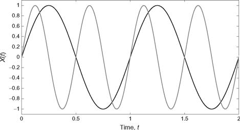
Figure 8.1 Member functions for the random process of Example 8.1.
Example 8.2
Now suppose that an experiment results in a random variable A that is uniformly distributed over [0,1). A random process is then constructed according to X(t) = A sin(ωo t). Since the random variable is continuous, there are an uncountably infinite number of realizations of the random process. A few are shown in Figure 8.2. As with the previous example, given an observation of the realization of the random process at one point in time, X(t1), one could determine the rest of the realization (as long as ωo t1 ≠ π).
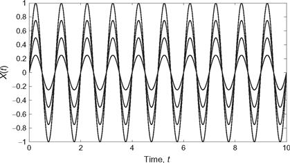
Figure 8.2 Some member functions for the random process of Example 8.2.
Example 8.3
This example is a generalization of that given in Example 8.1. Suppose now the experiment consists of flipping a coin repeatedly and observing the sequence of outcomes. The random process X(t) is then constructed as X(t) = sin(Ω i t), (i−1)T ≤ t ≤ iT, where Ω i = ωo if the ith flip of the coin results in “heads” and Ω i = 2ωo if the ith flip of the coin results in “tails.” One possible realization of this random process is illustrated in Figure 8.3. This is the sort of signal that might be produced by a frequency shift keying modem. In that application, the frequencies are not determined by coin tosses, but by random data bits instead.

Figure 8.3 One possible realization for the random process of Example 8.3.
Example 8.4
 As an example of a random process that is discrete in amplitude but continuous in time, we present the so-called “random telegraph” process. Let T1, T2, T3, … be a sequence of IID random variables, each with an exponential distribution,
![]()
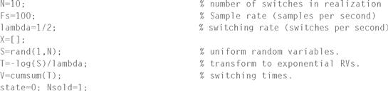
At any time instant, the random telegraph signal, X(t), takes on one of two possible states, X(t) = 0 or X(t) = 1. Suppose the process starts (at time t = 0) in the zero state. It then remains in that state for a time interval equal to T1 at which point it switches to the state X(t) = 1. The process remains in that state for another interval of time equal in length to T2 and then switches states again. The process then continues to switch after waiting for time intervals specified by the sequence of exponential random variables. One possible realization is shown in Figure 8.4. The MATLAB code for generating such a process follows.

Figure 8.4 One possible realization for the random telegraph signal of Example 8.4.
Example 8.5
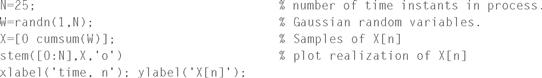
As an example of a discrete-time random process, suppose each outcome of an experiment produces a sequence of IID, zero-mean Gaussian random variables, W1, W2, W3, …. A discrete-time random process X[n] could be constructed according to:
![]()
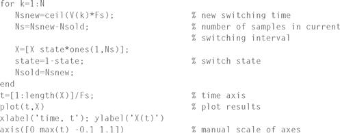
with the initial condition X[0] = 0. The value of the process at each point in time is equal to the value of the process at the previous point in time plus a random increase (decrease) which follows a Gaussian distribution. Note also that X[n] is just the sum of the first n terms in the sequence Wi . A sample realization of this random process is shown in Figure 8.5. The MATLAB code for generating this process is provided here.

Figure 8.5 One possible realization for the discrete-time random process of Example 8.5.
The reader is encouraged to run this program several times to see several different realizations of the same random process.
8.2 Mathematical Tools for Studying Random Processes
As with random variables, we can mathematically describe a random process in terms of a cumulative distribution function, probability density function, or a probability mass function. In fact, given a random process, X(t), which is sampled at some specified point in time, t = t k , the result is a random variable, Xk = X(tk ). This random variable can then be described in terms of its PDF, fX (xk ; tk ). Note that an additional time variable has been added to the PDF. This is necessary due to the fact that the PDF of the sample of the random process may depend on when the process is sampled. If desired, the CDF or PMF can be used rather than the PDF to describe the sample of the random process.
Example 8.6
Consider the random telegraph signal of Example 8.4. Since this process is binary valued, any sample will be a Bernoulli random variable. The only question is, what is the probability that X k = X(t k ) is equal to 1 (or 0)? Suppose that there are exactly n switches in the time interval [0, t k ). Then X(t k ) = n mod 2. Stated another way, define S n = T1 + T2+ … + T n . There will be exactly n switches in the time interval [0,t k ) provided that S n ≤ t k ≤ S n + 1. Therefore,
Since the T i are IID and exponential, S n will follow a Gamma distribution. Using the Gamma PDF for f s n (s) and the fact that Pr(T n +1 > t k − s) = exp(−λ(t k − s)) results in
![]()
So, it is seen that the number of switches in the interval [0, t k ) follows a Poisson distribution. The sample of the random process will be equal to 0 if the number of switches is even. Thus,
![]()
Likewise,
![]()
The behavior of this distribution as it depends on time is shown in Figure 8.6 and should make intuitive sense. For very small values of t k , it is most likely that there are no switches in the interval [0, t k ), in which case Pr(X(t k )=0) should be close to one. On the other hand, for large t k , many switches will likely occur and it should be almost equally likely that the process take on the values of 0 or 1.

Figure 8.6 Time dependence of the PMF for the random telegraph signal.
Example 8.7
Now consider the PDF of a sample of the discrete-time process of Example 8.5. Note that since X[n] is formed by summing n IID Gaussian random variables, X[n] will itself be a Gaussian random variable with mean of E[X[n]] = nμ W and variance Var(X[n]) = nσ2 w . In this case, since the W i ’s were taken to be zero-mean, the PDF of X[n] is
![]()
Once again, we see that for this example, the form of the PDF does indeed depend on when the sample is taken.
The PDF (or CDF or PMF) of a sample of a random process taken at an arbitrary point in time goes a long way toward describing the random process, but it is not a complete description. To see this, consider two samples, X1 = X(t1) and X2 = X(t2), taken at two arbitrary points in time. The PDF, fX (x; t), describes both X1 and X2, but it does not describe the relationship between X1 and X2. For some random processes, it might be reasonable to expect that X1 and X2 would be highly correlated if t1 is near t2, while X1 and X2 might be virtually uncorrelated if t1 and t2 are far apart. To characterize relationships of this sort, a joint PDF of the two samples would be needed. That is, it would be necessary to construct a joint PDF of the form f X1, X2 (x1, x2, t1, t2). This is referred to as a second-order PDF of the random process X(t).
Continuing with this reasoning, in order to completely describe the random process, it is necessary to specify an n th order PDF for an arbitrary n. That is, suppose the random process is sampled at time instants t1, t2, …, t n , producing the random variables X1 = X(t1), X2 = X(t2) …, X n = X(t n ). The joint PDF of the n samples, f X1, X2, …, X n (x1, x2, …,x n ; t1,t2, …, tn ), for an arbitrary n and arbitrary sampling times will give a complete description of the random process. In order to make this notation more compact, the vectors X = (X1, X2, …, Xn)T, x = (x1, x2, …, xn)T, and t = (t1, t2, …, tn)T are introduced and the nth order joint PDF is written as f X (x; t).
Unfortunately, for many realistic random processes, the prospects of writing down an n-th order PDF are rather daunting. One notable exception is the Gaussian random process which will be described in detail in Section 8.5. However, for most other cases, specifying a joint PDF of n samples may be exceedingly difficult, and hence it is necessary to resort to a simpler but less complete description of the random process. The simplest is the mean function of the process.
Definition 8.2: The mean function of a random process is simply the expected value of the process. For continuous time processes, this is written as
![]() (8.1)
(8.1)
while for discrete-time processes, the following notation is used:
![]() (8.2)
(8.2)
In general, the mean of a random process may change with time, but in many cases, this function is constant. Also, it is noted that only the first-order PDF of the process is needed to compute the mean function.
Example 8.8
Consider the random telegraph process of Example 8.4. It was shown in Example 8.6 that the first-order PMF of this process was described by a Bernoulli distribution with
![]()
The mean function then follows as
![]()
Example 8.9
Next, consider the sinusoidal random process of Example 8.2 where X(t) = A sin(ωo t) and A was a uniform random variable over [0,1). In this case,
![]()
This example illustrates a very important concept in that quite often it is not necessary to explicitly evaluate the first-order PDF of a random process in order to evaluate its mean function.
Example 8.10
Now suppose the random process of the previous example is slightly modified. In particular, consider a sine-wave process where the random variable is the phase, Θ which is uniformly distributed over [0, 2π). That is, X(t) = asin(ωo t+ Θ). For this example, the amplitude of the sine wave, a, is taken to be fixed (not random). The mean function is then
![]()
which is a constant. Why is the mean function of the previous example a function of time and this one is not? Consider the member functions of the respective ensembles for the two random processes.
Example 8.11
Now consider a sinusoid with a random frequency X{t) = cos(2πFt), where F is a random variable uniformly distributed over some interval (0,fo). The mean function can be readily determined to be
![]()
We can also estimate the mean function through simulation. Below we provide some MATLAB code to produce many realizations of this random process. The mean function is then found by taking the sample mean of all the realizations created. The sample mean and the ensemble mean are shown in Figure 8.7. Naturally, more or less accuracy in the sample mean can be obtained by varying the number of realizations generated.
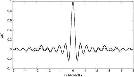
Figure 8.7 Comparison of the sample mean and ensemble mean for the sinusoid with random frequency of Example 8.11. The solid line is the sample mean while the dashed line is the ensemble mean.

To partially describe the second-order characteristics of a random process, the autocorrelation function is introduced.
Definition 8.3: The autocorrelation function, R XX (t1, t2), of a continuous-time random process, X(t), is defined as the expected value of the product X(t1)X(t2):
![]() (8.3)
(8.3)
For discrete-time processes, the autocorrelation function is
![]() (8.4)
(8.4)
Naturally, the autocorrelation function describes the relationship (correlation) between two samples of a random process. This correlation will depend on when the samples are taken; thus, the autocorrelation function is, in general, a function of two time variables. Quite often we are interested in how the correlation between two samples depends on how far apart the samples are spaced. To explicitly draw out this relationship, define a time difference variable, τ = t2−t1, and the autocorrelation function can then be expressed as
![]() (8.5)
(8.5)
where we have replaced tl with t to simplify the notation even further.
Example 8.12
Consider the sine wave process with a uniformly distributed amplitude as described in Examples 8.2 and 8.9, where X(t) = Asin(ωo t). The autocorrelation function is found as
![]()
or
![]()
Example 8.13
Now consider the sine wave process with random phase of Example 8.10 where X(t) = asin(ωo t+ Θ). Then
![]()
To aid in calculating this expected value, we use the trigonometric identity
![]()
The autocorrelation then simplifies to
![]()
or
![]()
Note that in this case, the autocorrelation function is only a function of the difference between the two sampling times. That is, it does not matter where the samples are taken, only how far apart they are.
Example 8.14
Recall the random process of Example 8.5 where X[n] = X[n − 1] + Wn , X[0] = 0 and the W n were a sequence of IID, zero-mean Gaussian random variables. In this case, it is easier to calculate the autocorrelation function using the alternative expression,
![]()
Then,
Since the Wi are IID and zero-mean, E[WiWj ] = 0 unless i = j. Therefore,
![]()
Definition 8.4: The autocovariance function, CXX (t1, t2), of a continuous time random process, X(t), is defined as the covariance of X(t1) and X(t2):
![]() (8.6)
(8.6)
The definition is easily extended to discrete-time random processes.
As with the covariance function for random variables, the autocovariance function can be written in terms of the autocorrelation function and the mean function:
![]() (8.7)
(8.7)
Once the mean and autocorrelation functions of a random process have been computed, the autocovariance function is trivial to find.
The autocovariance function is helpful when studying random processes which can be represented as the sum of a deterministic signal, s(t), plus a zero-mean noise process, N(t). If X(t) = s(t) +N(t), then the autocorrelation function of X(t) is
![]() (8.8)
(8.8)
using the fact that μN (t) = 0. If the signal is strong compared to the noise, the deterministic part will dominate the autocorrelation function, and thus Rxx (t1, t2) will not tell us much about the randomness in the process X(t). On the other hand, the autocovariance function is
![]() (8.9)
(8.9)
Therefore, the autocovariance function allows us to isolate the noise which is the source of randomness in the process.
Definition 8.5: For a pair of random processes X(t) and Y(t), the cross-correlation function is defined as
![]() (8.10)
(8.10)
Likewise, the cross-covariance function is
![]() (8.11)
(8.11)
Example 8.15
Suppose X(t) is a zero-mean random process with autocorrelation function Rxx (t1, t2). A new process Y(t) is formed by delaying X(t) by some amount td. That is, Y(t) = X(t−td). Then the cross-correlation function is
![]()
In a similar fashion, it is seen that RYX (t1, t2) = RXX (t1 − td, t2) and RYY (t1, t2) = RXX (t1 − td, t2 − td).
8.3 Stationary and Ergodic Random Processes
From the few simple examples given in the preceding section, we conclude that the mean function and the autocorrelation (or autocovariance) function can provide information about the temporal structure of a random process. We will delve into the properties of the autocorrelation function in more detail later in this chapter, but first the concepts of stationarity and ergodicity must be introduced.
Definition 8.6: A continuous time random process X(t) is strict sense stationary if the statistics of the process are invariant to a time shift. Specifically, for any time shift τ and any integer n ≥ 1,
 (8.12)
In general, it is quite difficult to show that a random process is strict sense stationary since to do so, one needs to be able to express the general nth order PDF. On the other hand, to show that a process is not strict sense stationary, one needs to show only that one PDF of any order is not invariant to a time shift. One example of a process that can be shown to be stationary in the strict sense is an IID process. That is, suppose X(t) is a random process that has the property that X(t) has an identical distribution for any t and that X(t1) and X(t2) are independent for any t1 ≠ t2. In this case,
![]() (8.13)
(8.13)
Since the nth order PDF is the product of first order PDFs and the first-order PDF is invariant to a time shift, then the nth order PDF must be invariant to a time shift.
Example 8.16
Consider the sinusoidal process with random amplitude from Example 8.2, where X(t) = Asin(ωo t). This process is clearly not stationary since if we take any realization of the process, x(t) = asin(ωo t), then a time shift x(t + τ) = asin(ωo(t + τ)) would not be a realization in the original ensemble. Now suppose the process has a random phase rather than a random amplitude as in Example 8.10, resulting in X(t) = asin(ωo t + Θ). It was already shown in Example 8.10 that μ X (t) = 0 for this process, and therefore the mean function is invariant to a time shift. Furthermore, in Example 8.13, it was shown that Rxx (t, t + τ) = (a2/2)cos(ωoτ), and thus the autocorrelation function is also invariant to a time shift. It is not difficult to show that the first-order PDF follows an arcsine distribution
![]()
and it is also independent of time and thus invariant to a time shift. It seems that this process might be stationary in the strict sense, but it would be rather cumbersome to prove it because the nth order PDF is difficult to specify.
As was seen in Example 8.16, it may be possible in some examples to determine that some of the statistics of a random process are invariant to time shifts, but determining stationarity in the strict sense may be too big of a burden. In those cases, we often settle for a looser form of stationarity.
Definition 8.7: A random process is wide sense stationary (WSS) if the mean function and autocorrelation function are invariant to a time shift. In particular, this implies that
![]() (8.14)
(8.14)
![]() (8.15)
(8.15)
All strict sense stationary random processes are also WSS, provided that the mean and autocorrelation function exist. The converse is not true. A WSS process does not necessarily need to be stationary in the strict sense. We refer to a process which is not WSS as non-stationary.
Example 8.17
Suppose we form a random process Y(t) by modulating a carrier with another random process, X(t). That is, let Y(t) = X(t)cos(ωo t + Θ) where Θ is uniformly distributed over [0, 2π) and independent of X(t). Under what conditions is Y(t) WSS? To answer this, we calculate the mean and autocorrelation function of Y(t).
While the mean function is a constant, the autocorrelation is not necessarily only a function of τ. The process Y(t) will be WSS provided that Rxx (t, t + τ) = Rxx (τ). Certainly if X(t) is WSS, then Y(t) will be as well.
Example 8.18
Let X(t) = At + B where A and B are independent random variables, both uniformly distributed over the interval (−1,1). To determine whether this process is WSS, calculate the mean and autocorrelation functions:

Clearly, this process is not WSS.
Many of the processes we deal with are WSS and hence have a constant mean function and an autocorrelation function that depends only on a single time variable. Hence, in the remainder of the text, when a process is known to be WSS or if we are assuming it to be WSS, then we will represent its autocorrelation function by RXX (τ). If a process is non-stationary or if we do not know if the process is WSS, then we will explicitly write the autocorrelation function as a function of two variables, RXX (t, t+ τ). For example, if we say that a process has a mean function of μ X = 1, and an autocorrelation function, RXX (τ) = exp(−|τ|), then the reader can infer that the process is WSS, even if it is not explicitly stated.
In order to calculate the mean or autocorrelation function of a random process, it is necessary to perform an ensemble average. In many cases, this may not be possible as we may not be able to observe all realizations (or a large number of realizations) of a random process. In fact, quite often we may be able to observe only a single realization. This would occur in situations where the conditions of an experiment cannot be duplicated and therefore the experiment is not repeatable. Is it possible to calculate the mean and/or autocorrelation function from a single realization of a random process? The answer is sometimes, depending on the nature of the process.
To start with, consider the mean. Suppose a WSS random process X(t) has a mean μX. We are able to observe one realization of the random process, x(t), and wish to try to determine μX from this realization. One obvious approach would be to calculate the time average1 of the realization:
 (8.16)
However, it is not obvious if the time average of one realization is necessarily equal to the ensemble average. If the two averages are the same, then we say that the random process is ergodic in the mean.
One could take the same approach for the autocorrelation function. Given a single realization, x(t), form the time-average autocorrelation function:
 (8.17)
If ℜ XX (τ) = Rxx (τ) for any realization, x(t), then the random process is said to be ergodic in the autocorrelation. In summary, we have the following definition of ergodicity:
Definition 8.8: A WSS random process is ergodic if ensemble averages involving the process can be calculated using time averages of any realization of the process. Two limited forms of ergodicity are:
• Ergodic in the mean − 〈x(t)〉 = E[X(t)],
• Ergodic in the autocorrelation − 〈x(t)x(t + τ)〉 = E[X(t)X(t + τ)].
Example 8.19
As a simple example, suppose X(t) = A where A is a random variable with some arbitrary PDF f A (a). Note that this process is stationary in the strict sense since for any realization, x(t) = x(t+ τ). That is, not only are the statistics of the process invariant to time shifts, but every realization is also invariant to any time shift. If we take the time average of a single realization, x(t) = a, we get 〈x(t)〉 = a. Hence, each different realization will lead to a different time average and will not necessarily give the ensemble mean, μA . Although this process is stationary in the strict sense, it is not ergodic in any sense.
Example 8.20
Now consider the sinusoid with random phase X(t) = asin(ωo t + Θ), where Θ is uniform over [0, 2π). It was demonstrated in Example 8.13 that this process is WSS. But is it ergodic? Given any realization x(t) = asin(ωo t+ θ), the time average is 〈x(t)〉 = 〈asin(ωo t+ θ)〉 = 0. That is, the average value of any sinusoid is zero. So, this process is ergodic in the mean since the ensemble average of this process was also zero. Next, consider the sample autocorrelation function:

This also is exactly the same expression obtained for the ensemble averaged autocorrelation function. Therefore, this process is also ergodic in the autocorrelation.
Example 8.21
For a process that is known to be ergodic, the autocorrelation function can be estimated by taking a sufficiently long time average of the autocorrelation function of a single realization. We demonstrate this via MATLAB for a process that consists of a sum of sinusoids of fixed frequencies and random phases,
![]()
where the θ K are IID and uniform over (0, 2π). For an arbitrary signal x(t), we note the similarity between the time-averaged autocorrelation function and the convolution of x(t) and x(−t). If we are given a single realization, x(t), which lasts only for the time interval, (−to, to), then these two expressions are given by
![]()
![]()
for τ>0. In general, we have the relationship
![]()
By using the MATLAB convolution function, conv, the time-averaged autocorrelation can easily be computed. This is demonstrated in the code that follows. Figure 8.8 shows a comparison between the ensemble averaged autocorrelation and the time-averaged autocorrelation taken from a single realization. From the figure, it is noted that the agreement between the two is good for τ« to, but not good when τ∼ to. This is due to the fact that when τ approaches to, the time window over which the time average is computed gets too small to produce an accurate estimate.

Figure 8.8 Comparison of the time-average autocorrelation and the ensemble-average autocorrelation for the sum of sinusoids process of Example 8.21. The solid line is the time-average autocorrelation while the dashed line is the ensemble-average autocorrelation.


The previous examples show two different random processes, one that is ergodic and one that is not. What characteristics of a random process make it ergodic? To get some better insight toward answering this question, consider a discrete-time process, X[n], where each random variable in the sequence is IID and consider forming the time average,
 (8.18)
The right hand side of the previous equation is nothing more than the sample mean. By virtue of the law of large numbers, the limit will indeed converge to the ensemble mean of the random process, μX , and thus this process is ergodic in the mean. In this case, the time average converges to the ensemble average because each time sample of the random process gives an independent observation of the underlying randomness. If the samples were highly correlated, then taking more samples would not necessarily cause the sample mean to converge to the ensemble mean. So, it seems that the form of the autocorrelation function will play some role in determining if a random process is ergodic in the mean.
To formalize this concept, consider the time average of an arbitrary WSS random process.
 (8.19)
Note that X to is a random variable with an expected value given by2
 (8.20)
Therefore, X to is an unbiased estimate of the true mean, but for the process to be ergodic in the mean, it is required that X to converges to μX as to→∞ This convergence will occur (in the mean square sense) if the variance of X to goes to zero in the limit as to→∞. To see under what conditions this occurs, we calculate the variance.
 (8.21)
Since the random process X(t) is WSS, the autocovariance is only a function of τ = t − s. As a result, the double integral can be converted to a single integral.3 The result is
 (8.22)
Thus, the random process will be ergodic in the mean if this expression goes to zero in the limit as to→0 This proves the following theorem.
Theorem 8.1: A continuous WSS random process X(t) will be ergodic in the mean if
 (8.23)
One implication of Theorem 8.1 is that if Cxx (τ) tends to a constant as τ→∞, then that constant must be zero for the process to be ergodic. Stated in terms of the autocorrelation function, a sufficient condition for a process to be ergodic in the mean is that
![]() (8.24)
(8.24)
Similar relationships can be developed to determine when a process is ergodic in the autocorrelation, but that topic is beyond the intended scope of this text.
Example 8.22
Consider the process X(t) = A of Example 8.19. It is easily found that the autocovariance function of this process is CXX (τ)=σ2 A for all τ. Plugging this into the left-hand side of Equation (8.23) results in
![]()
Since this limit is not equal to zero, the process clearly does not meet the condition for ergodicity. Next, consider the sinusoidal process of Example 8.20. In that case, the autocovariance function is Cxx (τ) = (a2/2)cos(ωoτ) and the left hand side of Equation (8.23) produces
![]()
So, even though this autocorrelation function does not approach zero in the limit as τ→0 (it oscillates), it still meets the condition for ergodicity.
8.4 Properties of the Autocorrelation Function
Since the autocorrelation function, along with the mean, is considered to be a principal statistical descriptor of a WSS random process, we will now consider some properties of the autocorrelation function. It should quickly become apparent that not just any function of τ can be a valid autocorrelation function.
Property 8.4.1: The autocorrelation function evaluated at τ = 0, RXX (0), is the average normalized power in the random process, X(t).
To clarify this, note that Rxx (0) = E[X2(t)]. Now suppose the random process X(t) was a voltage measured at some point in a system. For a particular realization, x(t), the instantaneous power would be p(t) = x2(t)/r, where r is the impedance in Ohms (Ω). The average power (averaged over all realizations in the ensemble) would then be Pavg = E[X2(t)]/r = Rxx (0)/r. If, on the other hand, X(t) were a current rather than a voltage, then the average power would be Pavg = RXX (0)r. From a systems level, it is often desirable not to concern ourselves with whether a signal is a voltage or a current. Accordingly, it is common to speak of a normalized power, which is the power measured using a 1Ω impedance. With r = 1, the two expression for average power are the same and equal to the autocorrelation function evaluated at zero.
Property 8.4.2: The autocorrelation function of a WSS random process is an even function; that is, R XX (τ) = R XX (−τ).
This property can easily be established from the definition of autocorrelation. Note that Rxx (−τ) = E[X(t)X(t−τ)]. Since X(t) is WSS, this expression is the same for any value of t. In particular, replace t in the previous expression with t + τ so that RXX (−τ) = E[X(t + τ)X(t)] = R xx (τ). As a result of this property, any function of τ which is not even cannot be a valid autocorrelation function.
Property 8.4.3: The autocorrelation function of a WSS random process is maximum at the origin; that is, |RXX (τ)| ≤ RXX (0) for all τ.
This property is established using the fact that for any two random variables, X and Y,
![]() (8.25)
(8.25)
This fact was previously demonstrated in the proof of Theorem 5.4. Letting X = X(t) and Y = X(t + τ) results in
![]() (8.26)
(8.26)
Taking square roots of both sides results in Property 8.4.3.
Property 8.4.4: If X(t) is ergodic and has no periodic components, then ![]() .
.
Property 8.4.5: If X(t) has a periodic component, then Rxx (τ) will have a periodic component with the same period.
From these properties, it is seen that an autocorrelation function can oscillate, can decay slowly or rapidly, and can have a non-zero constant component. As the name implies, the autocorrelation function is intended to measure the extent of correlation of samples of a random process as a function of how far apart the samples are taken.
8.5 Gaussian Random Processes
One of the most important classes of random processes is the Gaussian random process which is defined as follows.
Definition 8.9: A random process, X(t), for which any n samples, X1 = X(t1), X2 = X(t2), …, X n = X(t n ), taken at arbitrary points in time t1, t2, …, tn , form a set of jointly Gaussian random variables for any n = 1, 2, 3, … is a Gaussian random process.
In vector notation, the vector of n samples, X = [X1, X2, … X n ]T, will have a joint PDF given by
 (8.27)
As with any joint Gaussian PDF, all that is needed to specify the PDF is the mean vector and the covariance matrix. When the vector of random variables consists of samples of a random process, to specify the mean vector, all that is needed is the mean function of the random process, μX (t), since that will give the mean for any sample time. Similarly, all that is needed to specify the elements of the covariance matrix, C i, j, = Cov(X(ti ), X(t j ), would be the autocovariance function of the random process, CXX (t1, t2), or equivalently the autocorrelation function, RXX (t1, t2), together with the mean function. Therefore, the mean and autocorrelation functions provide sufficient information to specify the joint PDF for any number of samples of a Gaussian random process. Note that since any nth order PDF is completely specified by μX (t) and RXX (t1, t2), if a Gaussian random process is WSS, then the mean and autocorrelation functions will be invariant to a time shift and therefore any PDF will be invariant to a time shift. Hence, any WSS Gaussian random process is also stationary in the strict sense.
Example 8.23
Consider the random process X(t) = Acos(ωo t) +Bsin(ωo t), where A and B are independent, zero-mean Gaussian random variables with equal variances of σ2. This random process is formed as a linear combination of two Gaussian random variables, and therefore samples of this process are also Gaussian random variables. The mean and autocorrelation functions of this process are found as
Note that this process is WSS since the mean is constant and the autocorrelation function depends only on the time difference. Since the process is zero-mean, the first-order PDF is that of a zero-mean Gaussian random variable:
![]()
This PDF is independent of time as would be expected for a stationary random process. Now consider the joint PDF of two samples, X1 = X(t) and X2 =X(t+τ). Since the process is zero-mean, the mean vector is simply the all-zeros vector. The covariance matrix is then of the form
The joint PDF of the two samples would then be
![]()
Note once again that this joint PDF is dependent only on time difference, τ, and not on absolute time t. Higher order joint PDFs could be worked out in a similar manner.
Suppose we create a random process that jumps by an amount of ±δ units every Δt seconds. One possible realization of such a random process is illustrated in Figure 8.9. This proces is often referred to as a random walk. Mathematically, we can express this process as

Figure 8.9 One possible realization of a random walk process.
 (8.28)
where the Wk
are IID Bernoulli random variables with Pr(Wk
=1) = Pr(W
k
= −1) = 1/2 and  Note that the mean of this process is
 (8.29)
Next, consider a limiting form of the random walk where we let both the time between jumps, Δt, and the size of the jumps, δ, simultaneously go to zero. Then the process consists of an infinite number of infinitesimal jumps. As Δ→0, the number of terms in the series in Equation (8.28) becomes infinite, and by virtue of the central limit theorem, X(t) will follow a Gaussian distribution. Thus, we have created a zero-mean Gaussian random process.
Since the process is Gaussain, to complete the statistical characterization of this process, we merely need to find the covariance (or correlation) function. Assuming t2 > t1,
 (8.30)
To simplify the second term in the preceding equation, note that X(t1) represents the accumulation of jumps in the time interval [0, t1) while X(t2) − X(t1) represents the accumulation of jumps in the time interval [t1, t2). Due to the manner in which the process is constructed, these terms are independent, thus
![]() (8.31)
(8.31)
Therefore, R X,X (t1,t2) = E[X2(t1)] for t2 > t1. Similarly, if t1 > t2, we would find that R X,X (t1, t2) = E[X2(t2)]. From Equation (8.28), the variance of the process works out to be
 (8.32)
If we let δ → 0 and Δt → 0 in such a way that ![]() for some constant λ, then
for some constant λ, then
![]() (8.33)
(8.33)
and the covariance function is
![]() (8.34)
(8.34)
In principle, knowing the mean function and the covariance function of this Gaussian random process will allow us to specify the joint PDF of any number of samples.
This mathematical process is known as a Wiener process and finds applications in many different fields. It is perhaps most famously used to model Brownian motion which is the random fluctuation of minute particles suspended in fluids due to impact with neighboring atomic particles. It has also been used in the fields of finance, quantum mechanics, physical cosmology, and as will be seen in future chapters; in electrical engineering, the Weiner process is closely related to the commonly used white noise model of noise in electronic equipment.
8.6 Poisson Processes
Consider a process X(t) which counts the number of occurrences of some event in the time interval [0, t). The event might be the telephone calls arriving at a certain switch in a public telephone network, customers entering a certain store, or the birth of a certain species of animal under study. Since the random process is discrete (in amplitude), we will describe it in terms of a probability mass function, PX (i; t) = Pr(X(t) = i). Each occurrence of the event being counted is referred to as an arrival or a point. These types of processes are referred to as counting processes or birth processes. Suppose this random process has the following general properties:
• Independent Increments The number of arrivals in two non-overlapping intervals are independent. That is, for two intervals [t1, t2) and [t3, t4) such that t1 ≤ t2 ≤ t3 ≤ t4, the number of arrivals in [t1, t2) is statistically independent of the number of arrivals in [t3, t4).
• Stationary Increments The number of arrivals in an interval [t, t + τ) depends only on the length of the interval τ and not on where the interval occurs, t.
• Distribution of Infinitesimal Increments For an interval of infinitesimal length, [t, t + Δt), the probability of a single arrival is proportional to Δt, and the probability of having more than one arrival in the interval is negligible compared to Δt. Mathematically, we say that for some arbitrary constant λ:4
![]() (8.35)
(8.35)
![]() (8.36)
(8.36)
![]() (8.37)
(8.37)
Surprisingly enough, these rather general properties are enough to exactly specify the distribution of the counting process as shown next.
Consider the PMF of the counting process at time t + Δt. In particular, consider finding the probability of the event {X(t + Δt) = 0}.
 (8.38)
Subtracting P X (0; t) from both sides and dividing by Δt results in
![]() (8.39)
(8.39)
Passing to the limit as Δt → 0 gives the first-order differential equation
![]() (8.40)
(8.40)
The solution to this equation is of the general form
![]() (8.41)
(8.41)
for some constant c. The constant c is found to be equal to unity by using the fact that at time zero, the number of arrivals must be zero. That is PX (0;0) = 1. Therefore,
![]() (8.42)
(8.42)
The rest of the PMF for the random process X(t) can be specified in a similar manner. We find the probability of the general event {X(t + Δt) = i} for some integer i > 0.
P X (i; t + Δt) = Pr(i arrivals in [0, t)) Pr (no arrivals in [t, t + Δt))
+ Pr(i − 1 arrivals in [0, t))Pr(one arrival in [t, t + Δt))
+ Pr(less than i − 1 arrivals in [0, t)) Pr(more than One arrival in [t, t + Δt))
 (8.43)
As before, subtracting pX (i; t) from both sides and dividing by Δt results in
 (8.44)
Passing to the limit as Δt → 0 gives another first-order differential equation,
![]() (8.45)
(8.45)
It is fairly straightforward to solve this set of differential equations. For example, for i = 1 we have
![]() (8.46)
(8.46)
together with the initial condition that PX (1;0) = 0. The solution to this equation can be shown to be
![]() (8.47)
(8.47)
It is left as an exercise for the reader (see Exercise 8.32) to verify that the general solution to the family of differential equations specified in (8.45) is
![]() (8.48)
(8.48)
Starting with the three mild assumptions made about the nature of this counting process at the start of this section, we have demonstrated that X(t) follows a Poisson distribution, hence this process is referred to as a Poisson counting process. Starting with the PMF for the Poisson counting process specified in Equation (8.48), one can easily find the mean and autocorrelation functions for this process. First, the mean function is given by
 (8.49)
In other words, the average number of arrivals in the interval [0, t) is λt. This gives the parameter λ the physical interpretation of the average rate of arrivals, or as it is more commonly referred to the arrival rate of the Poisson process. Another observation we can make from the mean process is that the Poisson counting process is not stationary.
The autocorrelation function can be calculated as follows:
 (8.50)
To simplify the second expression, we use the independent increments property of the Poisson counting process. Assuming that t1 ≤ t2, then X(t1) represents the number of arrivals in the interval [0, t1), while X(t2) − X(t1) is the number of arrivals in the interval [t1, t2). Since these two intervals are non-overlapping, the number of arrivals in the two intervals are independent. Therefore,
 (8.51)
This can be written more concisely in terms of the autocovariance function,
![]() (8.52)
(8.52)
If t2 > t1, then the roles of t1 and t2 need to be reversed. In general for the Poisson counting process, we have
![]() (8.53)
(8.53)
Another feature that can be extracted from the PMF of the Poisson counting process is the distribution of the inter-arrival time. That is, let T be the time at which the first arrival occurs. We seek the distribution of the random variable T. The CDF of T can be found as
 (8.54)
Therefore, it follows that the arrival time is an exponential random variable with a mean value of E[T] = 1/λ. The PDF of T is
![]() (8.55)
(8.55)
We could get the same result starting from any point in time. That is, we do not need to measure the time to the next arrival starting from time zero. Picking any arbitrary point in time to, we could define T to be the time until the first arrival after time to. Using the same reasoning as above we would arrive at the same exponential distribution. If we pick to to be the time of a specific arrival, and then define T to be the time to the next arrival, then T is interpreted as an inter-arrival time. Hence, we conclude that the time between successive arrivals in the Poisson counting process follows an exponential distribution with a mean of 1/λ.
The Poisson counting process can be represented as a sum of randomly shifted unit step functions. That is, let Si be the time of the ith arrival. Then,
![]() (8.56)
(8.56)
The random variables, Si , are sometimes referred to as points of the Poisson process. Many other related random processes can be constructed by replacing the unit step functions with alternative functions. For example, if the step function is replaced by a delta function, the Poisson impulse process results, which is expressed as
![]() (8.57)
(8.57)
A sample realization of this process is shown in Figure 8.10.
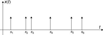
Figure 8.10 A sample realization of the Poisson impulse process.
8.7 Engineering Application—Shot Noise in a p–n Junction Diode
Both the Poisson counting process and the Poisson impulse process can be viewed as special cases of a general class of processes referred to as shot noise processes. Given an arbitrary waveform h(t) and a set of Poisson points, Si , the shot noise process is constructed as
![]() (8.58)
(8.58)
As an example of the physical origin of such a process, consider the operation of a p–n junction diode. When a forward bias voltage is applied to the junction, a current is generated. This current is not constant, but actually consists of discrete holes from the p region and electrons from the n region which have sufficient energy to overcome the potential barrier at the junction. Carriers do not cross the junction in a steady deterministic fashion; rather, each passage is a random event which might be modeled as a Poisson point process. The arrival rate of that Poisson process would be dependent on the bias voltage across the junction. As a carrier crosses the junction, it produces a current pulse, which we represent with some pulse shape h(t), such that the total area under h(t) is equal to the charge in an electron, q. Thus, the total current produced by the p–n junction diode can be modeled as a shot noise process.
To start with, we compute the mean function of a shot noise process. However, upon examining Equation (8.58), it is not immediately obvious how to take the expected value for an arbitrary pulse shape h (t). There are several ways to achieve the goal. One approach is to divide the time axis into infinitesimal intervals of length Δt. Then, define a sequence of Bernoulli random variables Vn such that Vn = 1 if a point occurred within the interval [n Δt, (n +1)Δt) and Vn = 0 if no points occurred in the same interval. Since the intervals are taken to be infinitesimal, the probability of having more than one point in a single interval is negligible. Furthermore, from the initial assumptions that led to the Poisson process, the distribution of the Vn is given by
![]() (8.59)
(8.59)
The shot noise process can be approximated by
![]() (8.60)
(8.60)
In the limit as Δt → 0, the approximation becomes exact. Using this alternative representation of the shot noise process, calculation of the mean function is straightforward.
![]() (8.61)
(8.61)
Note that in this calculation, the fact that E [Vn ] = λΔt was used. Passing to the limit as Δt → 0 results in
 (8.62)
Strictly speaking, the mean function of the shot noise process is not a constant, and therefore the process is not stationary. However, in practice, the current pulse will be time limited. Suppose the current pulse, h(t), has a time duration of th . That is, for t > t h , h(t) is essentially equal to zero. For the example of the p–n junction diode, the time duration of the current pulse is the time it takes the carrier to pass through the depletion region. For most devices, this number may be a small fraction of a nanosecond. Then for any t > t h ,
![]() (8.63)
(8.63)
For example, using the fact that the charge on an electron is 1.6 × 10⁻¹⁹C, if carriers made transitions at an average rate of 1015 per second (1 per femtosecond), then the average current produced in the diode would be 0.16 mA.
Next, we seek the autocorrelation (or autocovariance) function of the shot noise process. The same procedure used to calculate the mean function can also be used here.
 (8.64)
Passing to the limit as Δt → 0, we note that the term involving (λΔt)2 is negligible compared to λΔt. The resulting limit then takes the form
 (8.65)
Note that the last term (involving the product of integrals) is just the product of the mean function evaluated at time t and the mean function evaluated at time t+ τ. Thus, we have,
 (8.66)
or equivalently, in terms of the autocovariance function,
 (8.67)
As with the mean function, it is seen that the autocovariance function is a function of not only τ but also t. Again, for sufficiently large t, the upper limit in the preceding integral will be much longer than the time duration of the pulse, h (t). Hence, for t > th ,
![]() (8.68)
(8.68)
or
![]() (8.69)
(8.69)
We say that the shot noise process is asymptotically WSS. That is, after waiting a sufficiently long period of time, the mean and autocorrelation functions will be invariant to time shifts. In this case, the phrase “sufficiently long time” may mean a small fraction of a nanosecond! So for all practical purposes, the process is WSS. Also, it is noted that the width of the autocovariance function is th . That is, if h (t) is time limited to a duration of th , then CXX (τ) is zero for |τ| > th . This relationship is illustrated in Figure 8.11, assuming h(t) is a square pulse, and implies that any samples of the shot noise process that are separated by more than th will be uncorrelated.
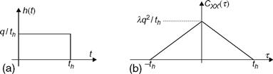
Figure 8.11 (a) A square current pulse and (b) the corresponding autocovariance function.
Finally, in order to characterize the PDF of the shot noise process, consider the approximation to the shot noise process given in Equation (8.60). At any fixed point in time, the process X(t) can be viewed as the linear combination of a large number of independent Bernoulli random variables. By virtue of the central limit theorem, this sum can be very well approximated by a Gaussian random variable. Since the shot noise process is WSS (at least in the asymptotic sense) and is a Gaussian random process, then the process is also stationary in the strict sense. Also, samples spaced by more than th are independent.
Example 8.24
Consider a shot noise process in a p–n junction diode where the pulse shape is square as illustrated in Figure 8.11. The mean current is μX = λq, which is presumably the desired signal we are trying to measure. The fluctuation of the shot noise process about the mean, we view as the unwanted disturbance, or noise. It would be interesting to measure the ratio of the power in the desired part of the signal to the power in the noise part of the signal. The desired part has a time-average power of μX 2 = (λq)2, while the noise part has a power of σ X 2 = C xx (0) = λq2/th . The signal-to-noise ratio (SNR) is then
![]()
We write this in a slightly different form,
![]()
For example, if the pulse duration were th = 10picoseconds, the SNR as it depends on the strength of the desired part of the signal would be as illustrated in Figure 8.12. It is noted that the SNR is fairly strong until we try to measure signals which are below a microamp.

Figure 8.12 Signal-to-noise ratio in a shot noise process for an example p–n junction diode.
In Chapter 10, we will view random processes in the frequency domain. Using the frequency domain tools we will develop in that chapter, it will become apparent that the noise power in the shot noise process is distributed over a very wide bandwidth (about 100 GHz for the previous example). Typically, our measuring equipment would not respond to that wide of a frequency range, and so the amount of noise power we actually see would be much less than that presented in Example 8.24 and would be limited by the bandwidth of our equipment.
Example 8.25
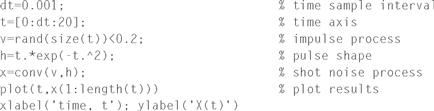
In this example, we provide some MATLAB code to generate a sample realization of a shot noise process. We chose to use a current pulse shape of the form, h(t) = texp(−t2), but the reader could easily modify this to use other pulse shapes as well. A typical realization is shown in Figure 8.13. Note that after a short initial transient period, the process settles into a steady-state behavior.

Figure 8.13 A typical realization of a shot noise process.
8.1 A discrete random process, X[n], is generated by repeated tosses of a coin. Let the occurrence of a head be denoted by 1 and that of a tail by −1. A new discrete random process is generated by Y[2n] = X[n] for n = 0, ±1,±2, … and Y[n] = X[n + 1] for n odd (either positive or negative). Find the autocorrelation function for Y[n].
8.2 Let Wn be an IID sequence of zero-mean Gaussian random variables with variance σ2 W . Define a discrete-time random process X[n] = pX[n − 1] + Wn , n = 1, 2, 3, …, where X[0] = W0 and p is a constant.
8.3 Let Xk
, k = 1, 2, 3, …, be a sequence of IID random variables with mean μX
and variance σ2
X
. Form the sample mean process
(a) Find the mean function, μs [n] = E[S[n]].
(b) Find the autocorrelation function, R s, s [k, n] = E[S[k]S[n]].
8.4 Define a random process according to
![]()
where X[0]= 0 and Wn is a sequence of IID Bernoulli random variables with Pr(Wn =1) = p and Pr(Wn = 0) = 1 − p.
(a) Find the PMF, PX (k; n) = Pr (X[k] = n).
(b) Find the joint PMF, P X1,X2 (k1, k2; n1, n2) = Pr(X[k1] = n1, X[k2] = n2).
(c) Find the mean function, μX [n] = E[X[n]].
(d) Find the autocorrelation function, R X,X [k, n] = E[X[k]X[n]].
8.5 Consider the random process defined in Example 8.5. The PDF, fX (x; n), and the mean function, μX [n], were found in Example 8.7.
8.6 A random process X(t) consists of three-member functions: X1 (t) = 1, X2(t) = −3, and x3 (t) = sin (2 πt). Each member function occurs with equal probability.
(a) Find the mean function, μX (t).
(b) Find the autocorrelation function, R X, X (t1, t2).
(c) Is the process WSS? Is it stationary in the strict sense?
8.7 A random process X(t) has the following member functions: x1(t) = −2cos(t), x2 (t) = −2sin (t), x3 (t) = 2 [cos (t) + sin (t)], x4(t) = [cos (t) −sin(t)], x5 (t) = [sin (t) −cos (t)]. Each member function occurs with equal probability.
(a) Find the mean function, μX (t).
(b) Find the autocorrelation function, R X, X (t1, t2).
(c) Is the process WSS? Is it stationary in the strict sense?
8.8 Let a discrete random process X[n] be generated by repeated tosses of a fair die. Let the values of the random process be equal to the results of each toss.
(a) Find the mean function, μX [n].
(b) Find the autocorrelation function, R X, X [k1, k2].
(c) Is the process WSS? Is it stationary in the strict sense?
8.9 Let X[n] be a wide sense stationary, discrete random process with autocorrelation function R X, X [n], and let c be a constant.
(a) Find the autocorrelation function for the discrete random process Y[n] = X[n] + c.
(b) Are X[n] and Y[n] independent? Uncorrelated? Orthogonal?
8.10 A wide sense stationary, discrete random process, X[n], has an autocorrelation function of R X, X [k]. Find the expected value of Y[n] = (X[n + m] −X[n − m])2, where m is an arbitrary integer.
8.11 A random process is given by X(t) = Acos (ωt) + B sin (ωt), where A and B are independent zero-mean random variables.
(a) Find the mean function, μX (t).
(b) Find the autocorrelation function, R X, X (t1, t2).
(c) Under what conditons (on the variances of A and B) is X(t) WSS?
8.12 Show by example that the random process Z(t) = X(t) + Y(t) may be a wide sense stationary process even though the random processes X(t) and Y(t) are not. Hint: Let A (t) and B (t) be independent, wide sense stationary random processes with zero-means and identical autocorrelation functions. Then let X(t) = A (t) sin (t) and Y(t) = B (t) cos (t). Show that X(t) and Y(t) are not wide sense stationary. Then show that Z(t) is wide sense stationary.
8.13 Let X(t) = A(t)cos(ω0 t + Θ), where A(t) is a wide sense stationary random process independent of Θ and let Θ be a random variable distributed uniformly over [0, 2 π). Define a related process Y(t) = A(t)cos((ω0 + ω1)t + Θ). Show that X(t) and Y(t) are stationary in the wide sense but that the cross-correlation R XY (t, t + τ), between X(t) and Y(t), is not a function of τ only and, therefore, Z(t) = X(t) + Y(t) is not stationary in the wide sense.
8.14 Let X(t) be a modified version of the random telegraph process. The process switches between the two states X(t) = 1 and X(t) = −1 with the time between switches following exponential distributions, fT (s) = λexp(−λs)u(s). Also, the starting state is determined by flipping a biased coin so that Pr(X(0)= 1) = p and Pr(X(0)=−1)= 1 − p.
(a) Find Pr(X(t) = 1) and Pr(X(t) = −1).
(b) Find the mean function, μX(t).
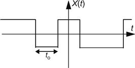
8.15 Let s(t) be a periodic square wave as illustrated in the accompanying figure. Suppose a random process is created according to X(t) = s (t − T), where T is a random variable uniformly distributed over (0, 1).
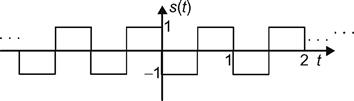
(a) Find the probability mass function of X(t).
(b) Find the mean function, μX (t).
8.16 Let s(t) be a periodic triangle wave as illustrated in the accompanying figure. Suppose a random process is created according to X(t) = s (t − T), where T is a random variable uniformly distributed over (0, 1).

(a) Find the probability mass function of X(t).
(b) Find the mean function, μX (t).
8.17 Let a random process consist of a sequence of pulses with the following properties: (i) the pulses are rectangular of equal duration, Δ (with no “dead” space in between pulses), (ii) the pulse amplitudes are equally likely to be ±1, (iii) all pulses amplitudes are statistically independent, and (iv) the various members of the ensemble are not synchronized.
8.18 A random process is defined by X(t) = exp(−At)u(t) where A is a random variable with PDF, fA (a).
(a) Find the PDF of X(t) in terms of fA (a).
(b) If A is an exponential random variable, with f A (a) = e−a u(a), find μ X (t) and R X,X (t1, t2). Is the process WSS?
8.19 Two zero-mean discrete-time random processes, X[n] and Y[n], are statistically independent. Let a new random process be Z[n] = X[n] + Y[n]. Let the autocorrelation functions for X[n] and Y[n] be
![]()
Find R
zz
[k]. Plot all three autocorrelation functions (you may want to use MATLAB to help).
8.20 Consider a discrete-time wide sense stationary random processes whose autocorrelation function is of the form
![]()
Assume this process has zero-mean. Is the process ergodic in the mean?
8.21 Let X(t) be a wide sense stationary random process that is ergodic in the mean and the autocorrelation. However, X(t) is not zero-mean. Let Y(t) = CX(t), where C is a random variable independent of X(t) and C is not zero-mean. Show that Y(t) is not ergodic in the mean or the autocorrelation.
8.22 Let X(t) be a WSS random process with mean μ
X
and autocorrelation function R
XX
(τ). Consider forming a new process according to

8.23 Which of the following could be the correlation function of a stationary random process?
8.24 A stationary random process, X(t), has a mean of μ X and correlation function, R X,X (τ). A new process is formed according to Y(t) = aX(t) + b for constants a and b. Find the correlation function R Y,Y (τ) in terms of μ X and R X,X (τ).
8.25 An ergodic random process has a correlation function given by
![]()
What is the mean of this process?
8.26 For each of the functions in Exercise 8.23 that represents a valid correlation function, construct a random process that possesses that function as its correlation function.
8.27 Let X(t) and Y(t) be two jointly wide sense stationary Gaussian random processes with zero-means and with autocorrelation and cross-correlation functions denoted as R XX (τ), R YY (τ), and R XY (τ). Determine the cross-correlation function between X2(t) and Y2 (t).
8.28 If X(t) is a wide sense stationary Gaussian random process, find the cross-correlation between X(t) and X3 (t) in terms of the autocorrelation function RXX (τ).
8.29 Suppose X(t) is a Weiner process with diffusion parameter λ = 1 as described in Section 8.5.
(a) Write the joint PDF of X1 = X(t1) and X2 = X(t2) for t2 > t1 by evaluating the covariance matrix of X = [X1, X2]T and using the general form of the joint Gaussian PDF in Equation 6.22.
(b) Evaluate the joint PDF of X1 = X(t1) and X2 = X(t2) for t2 > t1 indirectly by defining the related random variables Y1 = X1 and Y2 = X2 − X1. Noting that Y1 and Y2 are independent and Gaussian, write down the joint PDF of Y1 and Y2 and then form the joint PDF of X1 and X2 be performing the appropriate 2 × 2 transformation.
(c) Using the technique outlined in part (b), find the joint PDF of three samples of a Wiener process, X1 = X(t1), X2 = X(t2), and X3 = X(t3) for t1 ≤ t2 ≤ t3.
8.30 Let X(t) be a wide sense stationary Gaussian random process and form a new process according to Y(t) = X(t) cos (ωt + θ) where ω and θ are constants.
8.31 Let X(t) be a wide sense stationary Gaussian random process and form a new process according to Y(t) = X(t) cos (ωt + Θ) where ω is a constant and Θ is a random variable uniformly distributed over [0, 2π) and independent of X(t).
8.32 Prove that the family of differential equations,

leads to the Poisson distribution,
![]()
8.33 Consider a Poisson counting process with arrival rate λ.
(a) Suppose it is observed that there is exactly one arrival in the time interval [0, to). Find the PDF of that arrival time.
(b) Now suppose there were exactly two arrivals in the time interval [0, to). Find the joint PDF of those two arrival times.
(c) Extend these results to an arbitrary number, n, of arrivals?
8.34 Let N(t) be a Poisson counting process with arrival rate λ. Find Pr(N(t) = k|N(t + τ) = m) where τ> 0 and m ≥ k.
8.35 Let Xi
(t), i = 1, 2, …, n, be a sequence of independent Poisson counting processes with arrival rates, λ
i
. Show that the sum of all of these Poisson processes,

is itself a Poisson process. What is the arrival rate of the sum process?
8.36 A workstation is used until it fails and then it is sent out for repair. The time between failures, or the length of time the workstation functions until it needs repair, is a random variable T. Assume the times between failures, T1, T2, …, Tn of the workstations available are independent random variables that are identically distributed. For t > 0, let the number of workstations that have failed be N(t).
(a) If the time between failures of each workstation has an exponential PDF, then what type of process is N(t)?
(b) Assume that you have just purchased 10 new workstations and that each has a 90-day warranty. If the mean time between failures (MTBF) is 250 days, what is the probability that at least one workstation will fail before the end of the warranty period?
8.37 Suppose the arrival of calls at a switchboard is modeled as a Poisson process with the rate of calls per minute being λ a = 0.1.
(a) What is the probability that the number of calls arriving in a 10-minute interval is less than 10?
(b) What is the probability that the number of calls arriving in a 10-minute interval is less than 10 if λ a = 10?
(c) Assuming λ a = 0.1, what is the probability that one call arrives during the first 10-minute interval and two calls arrive during the second 10-minute interval?
8.38 Let X(t) be a Poisson counting process with arrival rate, λ. We form two related counting processes, Y1
t) and Y2 (t), by deterministically splitting the Poisson process, X(t). Each arrival associated with X(t) is alternately assigned to one of the two new processes. That is, if Si
is the ith arrival time of X(t), then

Find the PMFs of the two split processes, P
Y1
(k; t) = Pr(Y1(t) = k) and P
Y2
(k; t) = Pr (Y2(t) = k). Are the split processes also Poisson processes?
8.39 Let X(t) be a Poisson counting process with arrival rate, λ. We form two related counting processes, Y1(t) and Y2(t), by randomly splitting the Poisson process, X(t). In random splitting, the ith arrival associated with X(t) will become an arrival in process Y2 (t) with probability p and will become an arrival in process Y2(t) with probability 1 − p. That is, let Si
be the ith arrival time of X(t) and define Wi
to be a sequence of IID Bernoulli random variables with Pr(Wi
= 1) = p and Pr (Wi
= 0) = 1 − p. Then the split processes are formed according to
Find the PMFs of the two split processes, P
Y1
(k; t) = Pr(Y1(t) = k) and P
Y2
(k; t) = Pr(Y2(t) = k). Are the split processes also Poisson processes?
8.40 Consider a Poisson counting process with arrival rate, λ. Suppose it is observed that there have been exactly n arrivals in [0, t) and let S1, S2, Sn be the times of those n arrivals. Next, define X1,X2, …, Xn to be a sequence of IID random variables uniformly distributed over [0, t) and let Y1, Y2, Yn be the order statistics associated with the Xi . Show that the joint PDF of the order statistics, f Y (y), is identical to the joint PDF of the Poisson arrival times, f S (s). Hence, the order statistics are statistically identical to the arrival times.
8.41 Model lightning strikes to a power line during a thunderstorm as a Poisson impulse process. Suppose the number of lightning strikes in time interval t has a mean rate of arrival given by s, which is one strike per 3 minutes.
8.42 Suppose the power line in the previous problem has an impulse response that may be approximated by h(t) = te−at u(t), where a = 10s−1.
(a) What does the shot noise on the power line look like? Sketch a possible member function of the shot noise process.
(b) Find the mean function of the shot noise process.
(c) Find the autocorrelation function of the shot noise process.
8.43 A shot noise process with random amplitudes is defined by

where the Si are a sequence of points from a Poisson process and the Ai are IID random variables which are also indpendent of the Poisson points.
8.44 In this problem, we develop an alternative derivation for the mean function of the shot noise process described in Section 8.7,

where the Si
are the arrival times of a Poisson process with arrival rate, λ, and h (t) is an arbitrary pulse shape which we take to be causal. That is, h(t) = 0 for t ≤ 0. In order to find the mean function, μX
(t) = E[X(t)], we condition on the event that there were exactly n arrivals in [0, t). Then, the conditional mean function is

(a) Use the results of Exercise 8.40 to justify that
where the Xi are a sequence of IID random variables uniformly distributed over [0, t).
(b) Show that the expectation in part (a) reduces to
![]()
(c) Finally, average over the Poisson distribution of the number of arrivals to show that
![]()
8.45 Use the technique outlined in Exercise 8.44 to derive the autocovariance function of the shot noise process.
8.46 A random process X(t) is said to be mean square continuous at some point in time t, if
![]()
(a) Prove that X(t) is mean square continuous at time t if its correlation function, RX, X(t1, t2) is continuous at the point t1 = t, t2 = t.
(b) Prove that if X(t) is mean square continuous at time t, then the mean function μX(t) must be continuous at time t. Hint: Consider Var(X(t + to) − X(t)) and note that any variance must be non-negative.
(c) Prove that for a WSS process X(t), if RX, X(τ) is continuous at τ = 0, then X(t) is mean square continuous at all points in time.
8.47 Let N(t) be a Poisson counting process with arrival rate, λ. Determine whether or not N(t) is mean square continuous. Hint: See the definition of mean square continuity and the associated results in Exercise 8.46.
8.48 Let X(t) be a Weiner process with diffusion parameter λ as described in Section 8.5. Determine whether or not X(t) is mean square continuous. Hint: See the definition of mean square continuity and the associated results in Exercise 8.46.
8.49 Let Wk be a sequence of IID Bernoulli random variables with Pr (Wk = 1) = Pr(Wk= −1) = 1/2 and form a random process according to
where

A sample realization of this process is shown in the accompanying figure. Is this process mean square continuous? Hint: See the definition of mean square continuity and the associated results in Exercise 8.46.
8.50 You are given a member function of a random process as y(t) = 10sin(2π + π/2) where the amplitude is in volts. Quantize the amplitude of y(t) into 21 levels with the intervals ranging from − 10.5 to 10.5 in 1-volt steps. Consider 100 periods of y(t) and let t take on discrete values given by nts where ts = 5ms. Construct a histogram of y(t).
8.51 Write a MATLAB program to generate a Bernoulli process X[n] for which each time instant of the process is a Bernoulli random variable with Pr(X[n] = 1) = 0.1 and Pr(X[n] = 0) = 0.9. Also, the process is IID (i.e., X[n] is independent of X[m] for all m ≠ n). Once you have created the program to simulate X[n], then create a counting process Y[n] which counts the number of occurrences of X[m] = 1 in the interval m ∈ [0, n]. Plot member functions of each of the two processes.
8.52 Let Wn, n = 0, 1, 2, 3, …, be a sequence of IID zero-mean Gaussian random variables with variance σ2W = 1.
(a) Write a MATLAB program to generate the process
![]()
where X[0] = W0, and X[n] = 0 for n ≤ 0.
(b) Estimate the mean function of this process by generating a large number of realizations of the random process and computing the sample mean.
(c) Compute the time-averaged mean of the process from a single realization. Does this seem to give the same result as the ensemble mean estimated in part (b)?
8.53 A certain random process is created as a sum of a large number, n, of sinusoids with random frequencies and random phases,
where the random phases θk are IID and uniformly distributed over (0, 2 π) and the random frequencies are given by Fk = fo+ fdcos(βk), where the βk are IID and uniformly distributed over (0, 1). (Note: These types of processes occur in the study of wireless commuincation systems.) For this exercise, we will take the constants fo and fd to be fo = 25 Hz and fd = 10 Hz, while we will let the number of terms in the sum be n = 32.
(a) Write a MATLAB program to generate realizations of this random process.
(b) Assuming the process is stationary and ergodic, use a single realization to estimate the first-order PDF of the process, fX(x).
(c) Assuming the process is stationary and ergodic, use a single realization to estimate the mean of the process, μX.
(d) Assuming the process is stationary and ergodic, use a single realization to estimate the autocorrelation function of the process, RXX(τ).
8.54 Write a MATLAB program to generate a shot noise process with
![]()
where a = 1012s−1 and the constant b is chosen so that ![]() For this program, assume that carriers cross the depletion region at a rate of 1013 per second. Plot a member function of this random process.
For this program, assume that carriers cross the depletion region at a rate of 1013 per second. Plot a member function of this random process.
1 Throughout the text, angular brackets 〈 〉 are used as a shorthand notation to represent the time-average operator.
2 We exchange the order of expectation and integration since they are both linear operators.
3 The procedure for doing this conversion will be described in detail in Chapter 10, where a similar integral will be encountered in the proof of the Wiener-Khintchine-Einstein theorem.
4 The notation o(x) refers to an arbitrary function of x which goes to zero as x → 0 in a faster than linear fashion. That is, some function g(x) is said to be o(x) if ![]() .
.