CHAPTER 7
Random Sums and Sequences
This chapter forms a bridge between the study of random variables in the previous chapters and the study of random processes to follow. A random process is simply a random function of time. If time is discrete, then such a random function could be viewed as a sequence of random variables. Even when time is continuous, we often choose to sample waveforms (whether they are deterministic or random) in order to work with discrete time sequences rather than continuous time waveforms. Thus, sequences of random variables will naturally occur in the study of random processes. In this chapter, we will develop some basic results regarding both finite and infinite sequences of random variables and random series.
7.1 Independent and Identically Distributed Random Variables
In many applications, we are able to observe an experiment repeatedly. Each new observation can occur with an independent realization of whatever random phenomena control the experiment. This sort of situation gives rise to independent and identically distributed (IID or i.i.d.) random variables.
Definition 7.1: A sequence of random variables X1, X2, …, Xn is IID if
![]() (7.1)
(7.1)
and
 (7.2)
(7.2)
For continuous random variables, the CDFs can be replaced with PDFs in Equations (7.1) and (7.2), while for discrete random variables, the CDFs can be replaced by PMFs.
Suppose, for example, we wish to measure the voltage produced by a certain sensor. The sensor might be measuring the relative humidity outside. Our sensor converts the humidity to a voltage level which we can then easily measure. However, as with any measuring equipment, the voltage we measure is random due to noise generated in the sensor as well as in the measuring equipment. Suppose the voltage we measure is represented by a random variable X given by X = v(h) + N, where v(h) is the true voltage that should be presented by the sensor when the humidity is h, and N is the noise in the measurement. Assuming that the noise is zero-mean, then E[X] = v(h). That is, on the average, the measurement will be equal to the true voltage v(h). Furthermore, if the variance of the noise is sufficiently small, then the measurement will tend to be close to the true value we are trying to measure. But what if the variance is not small? Then the noise will tend to distort our measurement making our system unreliable. In such a case, we might be able to improve our measurement system by taking several measurements. This will allow us to “average out” the effects of the noise.
Suppose we have the ability to make several measurements and observe a sequence of measurements X1, X2, …, Xn It might be reasonable to expect that the noise that corrupts a given measurement has the same distribution each time (and hence the Xi are identically distributed) and is independent of the noise in any other measurement (so that the Xi are independent). Then the n measurements form a sequence of IID random variables. A fundamental question is then: How do we process an IID sequence to extract the desired information from it? In the preceding case, the parameter of interest, v(h), happens to be the mean of the distribution of the Xi. This turns out to be a fairly common problem and so we start by examining in some detail the problem of estimating the mean from a sequence of IID random variables.
7.1.1 Estimating the Mean of IID Random Variables
Suppose the Xi have some common PDF, fx (x), which has some mean value, μX. Given a set of IID observations, we wish to form some function,
![]() (7.3)
(7.3)
which will serve as an estimate of the mean. But what function should we choose? Even more fundamentally, what criterion should we use to select a function?
There are many criteria that are commonly used. To start with we would like the average value of the estimate of the mean to be equal to the true mean. That is, we want ![]() If this criterion is met, we say that
If this criterion is met, we say that ![]() is an unbiased estimate ofμX. Given that the estimate is unbiased, we would also like the error in the estimate to be as small as possible. Define the estimation error to be
is an unbiased estimate ofμX. Given that the estimate is unbiased, we would also like the error in the estimate to be as small as possible. Define the estimation error to be ![]() A common criterion is to choose the estimator which minimizes the second moment of the error (mean-square error),
A common criterion is to choose the estimator which minimizes the second moment of the error (mean-square error), ![]() If this criterion is met, we say that
If this criterion is met, we say that ![]() is an efficient estimator ofμX. To start with a relatively simple approach, suppose we desire to find a linear estimator. That is, we will limit ourselves to estimators of the form
is an efficient estimator ofμX. To start with a relatively simple approach, suppose we desire to find a linear estimator. That is, we will limit ourselves to estimators of the form
 (7.4)
(7.4)
Then, we seek to find the constants, a1, a2, …, an , such that the estimator (1) is unbiased and (2) minimizes the mean-square error. Such an estimator is referred to as the best linear unbiased estimator (BLUE).
To simplify notation in this problem, we write X = [Xl,
X2, …, Xn
]T and a = [ax, a2, …, an
]T. The linear estimator ![]() can then be written as
can then be written as ![]() First, for the estimator to be unbiased, we need
First, for the estimator to be unbiased, we need
![]() (7.5)
(7.5)
Since the Xi are all IID, they all have means equal to μX . Hence, the mean vector for X is just μX 1 n where 1 n is an n-element column vector of all ones. The linear estimator will then be unbiased if
 (7.6)
(7.6)
The mean square error is given by
 (7.7)
(7.7)
In this expression, R =E[XXT] is the correlation matrix for the vector X. Using the constraint of (7.6), the mean square error simplifies to
![]() (7.8)
(7.8)
The problem then reduces to minimizing the function aT Ra subject to the constraint aT 1n = 1.
To solve this multidimensional optimization problem, we use standard Lagrange multiplier techniques. Form the auxiliary function
![]() (7.9)
(7.9)
Then solve the equation ∇h = 0. It is not difficult to show that the gradient of the function h works out to be ∇h = 2Ra + λ 1 n . Therefore, the optimum vector a will satisfy
![]() (7.10)
(7.10)
Solving for a in this equation and then applying the constraint aT ln = 1 results in the solution
 (7.11)
Due to the fact that the Xi are IID, the form of the correlation matrix can easily be shown to be
![]() (7.12)
(7.12)
where I is an identity matrix and σ2 X is the variance of the IID random variables. It can be shown using the matrix inversion lemma1 that the inverse of this correlation matrix is
 (7.13)
From here, it is easy to demonstrate that R−1 1n is proportional to 1n, and therefore the resulting vector of optimum coefficients is
![]() (7.14)
(7.14)
In terms of the estimator ![]() , the best linear unbiased estimator of the mean of an IID sequence is
, the best linear unbiased estimator of the mean of an IID sequence is
 (7.15)
This estimator is commonly referred to as the sample mean. The preceding derivation proves Theorem 7.1 which follows.
Theorem 7.1: Given a sequence of IID random variables X1, X2, …, Xn , the sample mean is BLUE.
Another possible approach to estimating various parameters of a distribution is to use the maximum likelihood (ML) approach introduced in Chapter 6 (Section 6.5.2). In the ML approach, the distribution parameters are chosen to maximize the probability of the observed sample values occurring. Suppose, as in the preceding discussion, we are interested in estimating the mean of a distribution. Given a set of observations, X1 = x1, X2 = x2, …, Xn = xn , the ML estimate of μX would be the value of μX which maximizes fX (x). A few examples will clarify this concept.
Example 7.1
Suppose the Xi are jointly Gaussian so that

The value of μ which maximizes this expression will minimize
![]()
Differentiating and setting equal to zero gives the equation
![]()
The solution to this equation works out to be
![]()
Hence, the sample mean is also the ML estimate of the mean when the random variables follow a Gaussian distribution.
Example 7.2
Now suppose the random variables have an exponential distribution,
Differentiating with respect to μ and setting equal to zero results in

Solving for μ results in
![]()
Once again, the sample mean is the maximum likelihood estimate of the mean of the distribution.
Since the sample mean occurs so frequently, it is beneficial to study this estimator in a little more detail. First, we note that the sample mean is itself a random variable since it is a function of the n IID random variables. We have already seen that the sample mean is an unbiased estimate of the true mean; that is, ![]() . It is instructive to also look at the variance of this random variable.
. It is instructive to also look at the variance of this random variable.
 (7.16)
All terms in the double series in the previous equation are zero except for the ones where i = j since Xi and Xj are uncorrelated for all i ≠ j. Therefore, the variance of the sample mean is
 (7.17)
This means that if we use n samples to estimate the mean, the variance of the resulting estimate is reduced by a factor of n relative to what the variance would be if we used only one sample.
Consider what happens in the limit as n → ∞. As long as the variance of each of the samples is finite, the variance of the sample mean approaches zero. Of course, we never have an infinite number of samples in practice, but this does mean that the sample mean can achieve any level of precision (i.e., arbitrarily small variance) if a sufficient number of samples is taken. We will study this limiting behavior in more detail in a later section. For now, we turn our attention to estimating other parameters of a distribution.
7.1.2 Estimating the Variance of IID Random Variables
Now that we have a handle on how to estimate the mean of IID random variables, suppose we would like to also estimate the variance (or equivalently, the standard deviation). Since the variance is not a linear function of the random variables, it would not make much sense to try to form a linear estimator. That is, to talk about an estimator of the variance being BLUE is meaningless. Hence, we take the ML approach here. As with the problem of estimating the mean, we seek the value of the variance which maximizes the joint PDF of the IID random variables evaluated at their observed values.
Example 7.3
Suppose that the random variables are jointly Gaussian so that
Differentiating the joint PDF with respect to σ results in

Setting this expression equal to zero and solving results in
![]()
The result of Example 7.3 seems to make sense. The only problem with this estimate is that it requires knowledge of the mean in order to form the estimate. What if we do not know the mean? One obvious approach would be to replace the true mean in the previous result with the sample mean. That is, one could estimate the variance of an IID sequence using
 (7.18)
This approach, however, can lead to problems. It is left as an exercise for the reader to show that this estimator is biased; that is, in this case, E[2] ≠ σ2. To overcome this problem, it is common to adjust the previous form. The following estimator turns out to be an unbiased estimate of the variance:
 (7.19)
This is known as the sample variance and is the most commonly used estimate for the variance of IID random variables. In the previous expression, μ is the usual sample mean.
In summary, given a set of IID random variables, the variance of the distribution is estimated according to:
 (7.20)
Example 7.4
 Suppose we form a random variable Z according to Z =
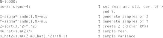
 ![]() where X and Y are independent Gaussian random variables with means of μ and variances of σ2. In this example, we will estimate the mean and variance of Z using the sample mean and sample variance of a large number of MATLAB-generated realizations of the random variable Z. The MATLAB code to accomplish this follows. Upon running this code, we obtained a sample mean of
where X and Y are independent Gaussian random variables with means of μ and variances of σ2. In this example, we will estimate the mean and variance of Z using the sample mean and sample variance of a large number of MATLAB-generated realizations of the random variable Z. The MATLAB code to accomplish this follows. Upon running this code, we obtained a sample mean of ![]() and a sample variance of
and a sample variance of ![]() . Note that the true mean and variance of the Rician random variable Z can be found analytically (with some effort). For this example, the PDF of the random variable Z is found to take on a Rician form
. Note that the true mean and variance of the Rician random variable Z can be found analytically (with some effort). For this example, the PDF of the random variable Z is found to take on a Rician form
![]()
Using the expressions given in Appendix D (see equations (D.52) and (D.53)) for the mean and variance of a Rician random variable, it is determined that the true mean and variance should be

For the values of μ = 2 and σ= 4 used in the following program, the resulting mean and variance of the Rician random variable should be μZ = 5.6211 and σ2Z = 8.4031.
7.1.3 Estimating the CDF of IID Random Variables
Suppose instead of estimating the parameters of a distribution, we were interested in estimating the distribution itself. This can be done using some of the previous results. The CDF of the underlying distribution is F X (x) = Pr (X ≤ x). For any specific value of x, define a set of related variables Y1, Y2, …, Yn such that
 (7.21)
It should be fairly evident that if the Xi are IID, then the Yi must be IID as well. Note that for these Bernoulli random variables, the mean is E[Yi ] = Pr(X ≤ x). Hence, estimating the CDF of the Xi is equivalent to estimating the mean of the Yi which is done using the sample mean
 (7.22)
This estimator is nothing more than the relative frequency interpretation of probability. To estimate F X (x) from a sequence of n IID observations, we merely count the number of observations that satisfy Xi ≤ x.
Example 7.5
To illustrate this procedure of estimating the CDF of IID random variables, suppose the X
i
are all uniformly distributed over (0, 1). The plot in Figure 7.1 shows the results of one realization of estimating this CDF using n IID random variables for n = 10, n = 100, and n = 1000. Clearly, as n gets larger, the estimate gets better. The MATLAB code that follows can be used to generate a plot similar to the one in Figure 7.1. The reader is encouraged to try different types of random variables in this program as well.

Figure 7.1 Estimate of the CDF of a uniform random variable obtained from n IID random variables, n=10, 100, and 1000.

7.2 Convergence Modes of Random Sequences
In many engineering applications, it is common to use various iterative procedures. In such cases, it is often important to know under what circumstances an iterative algorithm converges to the desired result. The reader is no doubt familiar with many such applications in the deterministic world. For example, suppose we wish to solve for the root of some equation g (x) = 0. One could do this with a variety of iterative algorithms (e.g., Newton’s method). The convergence of these algorithms is a quite important topic. That is, suppose xi is the estimate of the root at the ith iteration of Newton’s method. Does the sequence x1, x2, x3, … converge to the true root of the equation? In this section, we study the topic of random sequences and in particular the issue of convergence of random sequences.
As an example of a random sequence, suppose we started with a set of IID random variables, X1, X2, …, Xn, and then formed the sample mean according to
 (7.23)
The sequence S1,S2,S3,… is a sequence of random variables. It is desirable that this sequence converges to the true mean of the underlying distribution. An estimator satisfying this condition is called consistent. But in what sense can we say that the sequence converges? If a sequence of deterministic numbers S1, S2, S3, … was being considered, the sequence would be convergent to a fixed value s if
![]() (7.24)
(7.24)
More specifically, if for any ε>0, there exists an iε such that |si – s| ≤ ε for all i > iε, then the sequence is said to converge to s.
Example 7.6
Which of the following sequences converge in the limit as n → ∞?
For the sequence xn , |xn –0|≤ε will be satisfied provided that
![]()
Thus, the sequence xn
converges to ![]() . Likewise, for the sequence yn, |yn
–1| ≤ε will be satisfied provided that
. Likewise, for the sequence yn, |yn
–1| ≤ε will be satisfied provided that
![]()
In this case, the sequence yn
converges to ![]() . Finally, since the sequence zn
oscillates, there is no convergence.
. Finally, since the sequence zn
oscillates, there is no convergence.
Suppose an experiment, E, is run resulting in a realization, Z. Each realization is mapped to a particular sequence of numbers. For example, the experiment might be to observe a sequence of IID random variables X1,X2,X3, … and then map them into a sequence of sample means S1,S2,S3,…. Each realization, Z, leads to a specific deterministic sequence, some of which might converge (in the previous sense), while others might not converge. Convergence for a sequence of random variables is not straightforward to define and can occur in a variety of different manners.
7.2.1 Convergence Everywhere
The first and strictest form of convergence is what is referred to as convergence everywhere (a.k.a. sure convergence). A sequence is said to converge everywhere if every realization, ζ, leads to a sequence, S n (ζ), which converges to s(ζ). Note that the limit may depend on the particular realization. That is, the limit of the random sequence may be a random variable.
Example 7.7
Suppose we modify the deterministic sequence in part (a) of Example 7.6 to create a sequence of random variables. Let X be a random variable uniformly distributed over [0,1). Then define the random sequence
![]()
In this case, for any realization X = x, a deterministic sequence is produced of the form
![]()
which converges to ![]() . We say that the sequence converges everywhere (or surely) to
. We say that the sequence converges everywhere (or surely) to ![]() .
.
Example 7.8
Suppose we tried to modify the deterministic sequence in part (b) of Example 7.6 in a manner similar to what was done in Example 7.7. That is, let Y be a random variable uniformly distributed over [0, 1). Then define the random sequence
![]()
Now, for any realization Y = y, the deterministic sequence
![]()
converges to ![]() In this case, the value that the sequence converges to depends on the particular realization of the random variable Y. In other words, the random sequence converges to a random variable, lim
In this case, the value that the sequence converges to depends on the particular realization of the random variable Y. In other words, the random sequence converges to a random variable, lim ![]()
7.2.2 Convergence Almost Everywhere
In many examples, it may be possible to find one or several realizations of the random sequence which do not converge, in which case the sequence (obviously) does not converge everywhere. However, it may be the case that such realizations are so rare that we might not want to concern ourselves with such cases. In particular, suppose that the only realizations that lead to a sequence which does not converge occur with probability zero. Then we say the random sequence converges almost everywhere (a.k.a. almost sure convergence or convergence with probability 1). Mathematically, let A be the set of all realizations that lead to a convergent sequence. Then the sequence converges almost everywhere if Pr (A) = 1.
Example 7.9
As an example of a sequence that converges almost everywhere, consider the random sequence
![]()
where Z is a random variable uniformly distributed over [0,1). For almost every realization Z = z, the deterministic sequence
![]()
converges to ![]() . The one exception is the realization Z =0 in which case the sequence becomes zn
= 1 which converges, but not to the same value. Therefore, we say that the sequence Zn
converges almost everywhere (or almost surely) to lim
. The one exception is the realization Z =0 in which case the sequence becomes zn
= 1 which converges, but not to the same value. Therefore, we say that the sequence Zn
converges almost everywhere (or almost surely) to lim ![]() since the one exception to this convergence occurs with zero probability; that is, Pr(Z = 0) = 0.
since the one exception to this convergence occurs with zero probability; that is, Pr(Z = 0) = 0.
7.2.3 Convergence in Probability
A random sequence S1,S2,S3,. converges in probability to a random variable S if for any ε > 0,
![]() (7.25)
(7.25)
Example 7.10
Let Xk , k = 1, 2, 3, …, be a sequence of IID Gaussian random variables with mean μ and variance σ2. Suppose we form the sequence of sample means
![]()
Since the Sn are linear combinations of Gaussian random variables, then they are also Gaussian with E[Sn ] = μ and Var(Sn ) = σ2 /n. Therefore, the probability that the sample mean is removed from the true mean by more than ε is
![]()
As n → ∞, this quantity clearly approaches zero, so that this sequence of sample means converges in probability to the true mean.
7.2.4 Convergence in the Mean Square Sense
A random sequence S1,S2,S3, … converges in the mean square (MS) sense to a random variable S if
![]() (7.26)
(7.26)
Example 7.11
Consider the sequence of sample means of IID Gaussian random variables described in Example 7.10. This sequence also converges in the MS sense since
![]()
This sequence of sample variances converges to 0 as n → ∞ thus producing convergence of the random sequence in the MS sense.
7.2.5 Convergence in Distribution
Suppose the sequence of random variables S1, S2, S3, … has CDFs given by FSn (s) and the random variable S has a CDF, F s (s). Then, the sequence converges in distribution if
![]() (7.27)
(7.27)
for any s which is a point of continuity of FS (s).
Example 7.12
Consider once again the sequence of sample means of IID Gaussian random variables described in Example 7.10. Since Sn is Gaussian with mean μ and variance σ2 /n, its CDF takes the form
![]()
For any s > μ, ![]() , while for any s≤μ,
, while for any s≤μ, ![]() . Thus, the limiting form of the CDF is
. Thus, the limiting form of the CDF is
![]()
where u(s) is the unit step function. Note that the point s = μ is not a point of continuity of Fs (s) and therefore we do not worry about it for this proof.
It should be noted, as was seen in the previous sequence of examples, that some random sequences converge in many of the different senses. In fact, one form of convergence may necessarily imply convergence in several other forms. Table 7.1 illustrates these relationships. For example, convergence in distribution is the weakest form of convergence and does not necessarily imply any of the other forms of convergence. Conversely, if a sequence converges in any of the other modes presented, it will also converge in distribution. The reader will find a number of exercises at the end of the chapter which will illustrate and/or prove some of the relationships in Table 7.1.
Table 7.1. Relationships between convergence modes
 |
7.3 The Law of Large Numbers
Having described the various ways in which a random sequence can converge, we return now to the study of sums of random variables. In particular, we look in more detail at the sample mean. The following very well-known result is known as the weak law of large numbers.
Theorem 7.2 (The Weak Law of Large Numbers): Let Sn be the sample mean computed from n IID random variables, X1,X2, …, Xn . The sequence of sample means, Sn, converges in probability to the true mean of the underlying distribution, FX (x).
Proof: Recall that if the distribution F X (x) has a mean of μ and variance σ2, then the sample mean, Sn , has mean μ and variance σ2 /n. Applying Chebyshev’s inequality,
![]() (7.28)
(7.28)
Hence, ![]() for any ε> 0. Thus, the sample mean converges in probability to the true mean.
for any ε> 0. Thus, the sample mean converges in probability to the true mean.
The implication of this result is that we can estimate the mean of a random variable with any amount of precision with arbitrary probability if we use a sufficiently large number of samples. A stronger result known as the strong law of large numbers shows that the convergence of the sample mean is not just in probability but also almost everywhere. We do not give a proof of this result in this text.
As was demonstrated in Section 7.1.3, the sample mean can be used to estimate more than just means. Suppose we are interested in calculating the probability that some event A results from a given experiment. Assuming that the experiment is repeatable and each time the results of the experiment are independent of all other trials, then Pr(A) can easily be estimated. Simply define a random variable Xi that is an indicator function for the event A on the ith trial. That is, if the event A occurs on the ith trial, then Xi = 1, otherwise Xi = 0. Then
![]() (7.29)
(7.29)
The sample mean,
 (7.30)
will give an unbiased estimate of the true probability, Pr (A). Furthermore, the law of large numbers tells us that as the sample size gets large, the estimate will converge to the true value.
The weak law of large numbers tells us that the convergence is in probability while the strong law of large numbers tells us that the convergence is also almost everywhere.
The technique we have described for estimating the probability of events is known as Monte Carlo simulation. It is commonly used, for example, to estimate the bit error probability of a digital communication system. A program is written to simulate transmission and detection of data bits. After a large number of data bits have been simulated, the number of errors are counted and divided by the total number of bits transmitted. This gives an estimate of the true probability of bit error of the system. If a sufficiently large number of bits are simulated, arbitrary precision of the estimate can be obtained.
Example 7.13
This example shows how the sample mean and sample variance converges to the true mean for a few different random variables. The results of running the MATLAB code that follows are shown in Figure 7.2. Plot (a) shows the results for a Gaussian distribution, whereas plot (b) shows the same results for an arcsine random variable. In each case, the parameters have been set so that the true mean is μ = 3 and the variance of each sample is 1. Since the variance of the sample mean depends only on the variance of the samples and the number of samples, crudely speaking the “speed” of convergence should be about the same in both cases.

Figure 7.2 Convergence of the sample mean for (a) Gaussian and (b) Arcsine random variables.

7.4 The Central Limit Theorem
Probably the most important result dealing with sums of random variables is the central limit theorem which states that under some mild conditions, these sums converge to a Gaussian random variable in distribution. This result provides the basis for many theoretical models of random phenomena. It also explains why the Gaussian random variable is of such great importance and why it occurs so frequently. In this section, we prove a simple version of the Central Limit Theorem and then discuss some of the generalizations.
Theorem 7.3 (The Central Limit Theorem): Let Xi be a sequence of IID random variables with mean μX and variance σ2X. Define a new random variable, Z, as a (shifted and scaled) sum of the Xi :
 (7.31)
Note that Z has been constructed such that E[Z] = 0 and Var(Z) =1. In the limit as n approaches infinity, the random variable Z converges in distribution to a standard normal random variable.
Proof: The most straightforward approach to prove this important theorem is using characteristic functions. Define the random variable ![]() as
as ![]() . The characteristic function of Z is computed as
. The characteristic function of Z is computed as
 (7.32)
Next, recall Taylor’s theorem2 which states that any function g(x) can be expanded in a power series of the form
 (7.33)
where the remainder rk (x, xo) is small compared to (x – xo)k as x → xo. Applying the Taylor series expansion about the point ω = 0 to the characteristic function of X results in
![]() (7.34)
(7.34)
where r3(ω) is small compared to ω2 as ω → 0. Furthermore, we note that ![]() , and
, and ![]() Therefore, Equation (7.34) reduces to
Therefore, Equation (7.34) reduces to
![]() (7.35)
(7.35)
The characteristic function of Z is then
![]() (7.36)
(7.36)
Note that as n → ∞, the argument of r3 ( ) goes to zero for any finite ω. Thus, as ![]() becomes negligible compared to ω2/n. Therefore, in the limit, the characteristic function of Z approaches3
becomes negligible compared to ω2/n. Therefore, in the limit, the characteristic function of Z approaches3
![]() (7.37)
(7.37)
This is the characteristic function of a standard normal random variable.
Several remarks about this theorem are in order at this point. First, no restrictions were put on the distribution of the Xi . The preceding proof applies to any infinite sum of IID random variables, regardless of the distribution. Also, the central limit theorem guarantees that the sum converges in distribution to Gaussian, but this does not necessarily imply convergence in density. As a counter example, suppose that the Xi are discrete random variables, then the sum must also be a discrete random variable. Strictly speaking, the density of Z would then not exist, and it would not be meaningful to say that the density of Z is Gaussian. From a practical standpoint, the probability density of Z would be a series of impulses. While the envelope of these impulses would have a Gaussian shape to it, the density is clearly not Gaussian. If the Xi are continuous random variables, the convergence in density generally occurs as well.
The proof of the central limit theorem given above assumes that the Xi are IID. This assumption is not needed in many cases. The central limit theorem also applies to independent random variables that are not necessarily identically distributed. Loosely speaking4, all that is required is that no term (or small number of terms) dominates the sum, and the resulting infinite sum of independent random variables will approach a Gaussian distribution in the limit as the number of terms in the sum goes to infinity. The central limit theorem also applies to some cases of dependent random variables, but we will not consider such cases here.
From a practical standpoint, the central limit theorem implies that for the sum of a sufficiently large (but finite) number of random variables, the sum is approximately Gaussian distributed. Of course, the goodness of this approximation depends on how many terms are in the sum and also the distribution of the individual terms in the sum. The next examples show some illustrations to give the reader a feel for the Gaussian approximation.
Example 7.14
Suppose the Xi are all independent and uniformly distributed over (–1/2,1/2). Consider the sum
![]()
The sum has been normalized so that Z has zero-mean and unit variance. It was shown previously that the PDF of the sum of independent random variables is just the convolution of the individual PDFs. Hence, if we define Y = X1+X2+ … +X n then
![]()
The results of performing this n-fold convolution are shown in Figure 7.3 for several values of n. Note that for as few as n = 4 or n = 5 terms in the series, the resulting PDF of the sum looks very much like the Gaussian PDF.

Figure 7.3 PDF of the sum of independent uniform random variables: (a) n = 2, (b) n = 3, (c) n = 4, and (d) n = 5.
Example 7.15
In this example, suppose the Xi are now discrete Bernoulli distributed random variables such that Pr(Xi =1) = Pr(Xi =0) = 0.5. In this case, the sum Y = X1+X2+… +X n is a binomial random variable with PMF given by
![]()
The corresponding CDF is
![]()
The random variable Y has a mean of E[Y] = n/2 and variance of Var(Y) = n/4. In Figure 7.4, this binomial distribution is compared to a Gaussian distribution with the same mean and variance. It is seen that for this discrete random variable, many more terms are needed in the sum before good convergence to a Gaussian distribution is achieved.
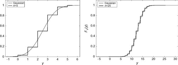
Figure 7.4 CDF of the sum of independent Bernoulli random variables; n = 5, 25.
7.5 Confidence Intervals
Consider once again the problem of estimating the mean of a distribution from n IID observations. When the sample mean ![]() is formed, what have we actually learned? Loosely speaking, we might say that our best guess of the true mean is
is formed, what have we actually learned? Loosely speaking, we might say that our best guess of the true mean is ![]() . However, in most cases, we know that the event
. However, in most cases, we know that the event ![]() occurs with zero probability (since if
occurs with zero probability (since if ![]() is a continuous random variable, the probability of it taking on any point value is zero). Alternatively, it could be said that (hopefully) the true mean is “close” to the sample mean. While this is a vague statement, with the help of the central limit theorem, we can make the statement mathematically precise.
is a continuous random variable, the probability of it taking on any point value is zero). Alternatively, it could be said that (hopefully) the true mean is “close” to the sample mean. While this is a vague statement, with the help of the central limit theorem, we can make the statement mathematically precise.
If a sufficient number of samples are taken, the sample mean can be well approximated by a Gaussian random variable with a mean of ![]() and
and ![]() . Using the Gaussian distribution, the probability of the sample mean being within some amount ε of the true mean can be easily calculated,
. Using the Gaussian distribution, the probability of the sample mean being within some amount ε of the true mean can be easily calculated,
![]() (7.38)
(7.38)
Stated another way, let εα be the value of ε such that the right hand side of the above equation is 1 – α; that is,
![]() (7.39)
(7.39)
where Q−1 () is the inverse of the Q-function. Then, given n samples which lead to a sample mean ![]() , the true mean will fall in the interval
, the true mean will fall in the interval ![]() with probability 1 – α. The interval
with probability 1 – α. The interval ![]() is referred to as the confidence interval while the probability 1 – α is the confidence level or, alternatively, α is the level of significance. The confidence level and level of significance are usually expressed as percentages. The corresponding values of the quantity cα
= Q−1 (α/2) are provided in Table 7.2 for several typical values of α. Other values not included in the table can be found from tables of the Q-function (such as provided in Appendix E).
is referred to as the confidence interval while the probability 1 – α is the confidence level or, alternatively, α is the level of significance. The confidence level and level of significance are usually expressed as percentages. The corresponding values of the quantity cα
= Q−1 (α/2) are provided in Table 7.2 for several typical values of α. Other values not included in the table can be found from tables of the Q-function (such as provided in Appendix E).
Table 7.2. Constants used to calculate confidence intervals
| Percentage of Confidence Level (1−α)*100% | Percentage of Level of Significance α*100% | |
| 90 | 10 | 1.64 |
| 95 | 5 | 1.96 |
| 99 | 1 | 2.58 |
| 99.9 | 0.1 | 3.29 |
| 99.99 | 0.01 | 3.89 |
Example 7.16
Suppose the IID random variables each have a variance of ![]() . A sample of n = 100 values is taken and the sample mean is found to be
. A sample of n = 100 values is taken and the sample mean is found to be ![]() . Determine the 95% confidence interval for the true mean μX
. In this case,
. Determine the 95% confidence interval for the true mean μX
. In this case, ![]() and the appropriate value of cα
is c0.05 = 1.96 from Table 7.2. The 95% confidence interval is then
and the appropriate value of cα
is c0.05 = 1.96 from Table 7.2. The 95% confidence interval is then
![]()
Example 7.17
Looking again at Example 7.16, suppose we want to be 99 % confident that the true mean falls within a factor of ±0.5 of the sample mean. How many samples need to be taken in forming the sample mean? To ensure this level of confidence, it is required that
![]()
and therefore
![]()
Since n must be an integer, it is concluded that at least 107 samples must be taken.
In summary, to achieve a level of significance specified by α, we note that by virtue of the central limit theorem, the sum
 (7.40)
approximately follows a standard normal distribution. We can then easily specify a symmetric interval about zero in which a standard normal random variable will fall with probability 1 – α. As long as n is sufficiently large, the original distribution of the IID random variables does not matter.
Note that in order to form the confidence interval as specified, the standard deviation of the Xi must be known. While in some cases, this may be a reasonable assumption, in many applications, the standard deviation is also unknown. The most obvious thing to do in that case would be to replace the true standard deviation in Equation (7.40) with the sample standard deviation. That is, we form a statistic
 (7.41)
and then seek a symmetric interval about zero (–tα,
tα) such that the probability that ![]() falls in that interval is 1 – α. For very large n, the sample standard deviation will converge to the true standard deviation and hence
falls in that interval is 1 – α. For very large n, the sample standard deviation will converge to the true standard deviation and hence ![]() will approach
will approach ![]() . Hence, in the limit as
. Hence, in the limit as ![]() can be treated as having a standard normal distribution, and the confidence interval is found in the same manner we have described. That is, as
can be treated as having a standard normal distribution, and the confidence interval is found in the same manner we have described. That is, as ![]() For values of n that are not very large, the actual distribution of the statistic
For values of n that are not very large, the actual distribution of the statistic ![]() must be calculated in order to form the appropriate confidence interval.
must be calculated in order to form the appropriate confidence interval.
Naturally, the distribution of ![]() will depend on the distribution of the Xi
. One case where this distribution has been calculated for finite n is when the Xi
are Gaussian random variables. In this case, the statistic
will depend on the distribution of the Xi
. One case where this distribution has been calculated for finite n is when the Xi
are Gaussian random variables. In this case, the statistic ![]() follows the so-called Student’s t-distribution5 with n – 1 degrees of freedom:
follows the so-called Student’s t-distribution5 with n – 1 degrees of freedom:
![]() (7.42)
(7.42)
where Γ( ) is the gamma function (see Chapter 3, Equation (3.22) or ">Appendix E, Equation (E.39)).
From this PDF, one can easily find the appropriate confidence interval for a given level of significance, α, and sample size, n. Tables of the appropriate confidence interval, tα, can be found in any text on statistics. It is common to use the t-distribution to form confidence intervals even if the samples are not Gaussian distributed. Hence, the t-distribution is very commonly used for statistical calculations.
Many other statistics associated with related parameter estimation problems are encountered and have been carefully expounded in the statistics literature. We believe that with the probability theory developed to this point, the motivated student can now easily understand the motivation and justification for the variety of statistical tests that appear in the literature. Several exercises at the end of this chapter walk the reader through some of the more commonly used statistical distributions including the t-distribution of Equation (7.42), the chi-square distribution (see Chapter 3, Section 3.4.6), and the F-distribution (see Appendix D).
Example 7.18
Suppose we wish to estimate the failure probability of some system. We might design a simulator for our system and count the number of times the system fails during a long sequence of operations of the system. Examples might include bit errors in a communication system, defective products in an assembly line, etc. The failure probability can then be estimated as discussed at the end of Section 7.3. Suppose the true failure probability is p (which of course is unknown to us). We simulate operation of the system n times and count the number of errors observed, Ne. The estimate of the true failure probability is then just the relative frequency,
![]()
If errors occur independently, then the number of errors we observe in n trials is a binomial random variable with parameters n and p. That is,
![]()
From this, we infer that the mean and variance of the estimated failure probability is ![]() and
and ![]() . From this, we can develop confidence intervals for our failure probability estimates. The MATLAB code that follows creates estimates as described and plots the results, along with error bars indicating the confidence intervals associated with each estimate. The plot resulting from running this code is shown in Figure 7.5.
. From this, we can develop confidence intervals for our failure probability estimates. The MATLAB code that follows creates estimates as described and plots the results, along with error bars indicating the confidence intervals associated with each estimate. The plot resulting from running this code is shown in Figure 7.5.

Figure 7.5 Estimates of failure probabilities along with confidence intervals. The solid line is the true probability while the circles represent the estimates.

7.6 Random Sums of Random Variables
The sums of random variables considered up to this point have always had a fixed number of terms. Occasionally, one also encounters sums of random variables where the number of terms in the sum is also random. For example, a node in a communication network may queue packets of variable length while they are waiting to be transmitted. The number of bytes in each packet, Xi, might be random as well as the number of packets in the queue at any given time, N. The total number of bytes stored in the queue would then be a random sum of the form
 (7.43)
Theorem 7.4: Given a set of IID random variables Xi with mean μX and variance σ2 X and an independent random integer N, the mean and variance of the random sum of the form given in Equation (7.43) are given by
![]() (7.44)
(7.44)
![]() (7.45)
(7.45)
Proof: To calculate the statistics of S, it is easier to first condition on N and then average the resulting conditional statistics with respect to N. To start with, consider the mean:
 (7.46)
The variance is found following a similar procedure. The second moment of S is found according to
 (7.47)
Note that Xi and Xj are uncorrelated unless i= j. Therefore, this expected value works out to be
![]() (7.48)
(7.48)
Finally, using Var(S) = E[s2]-(E[S])2 results in
![]() (7.49)
(7.49)
One could also derive formulas for higher order moments in a similar manner.
Theorem 7.5: Given a set of IID random variables Xi with a characteristic function ΦX (ω) and an independent random integer N with a probability generating function HN (z), the characteristic function of the random sum of the form given in Equation (7.43) is given by
![]() (7.50)
(7.50)
Proof: Following a derivation similar to the last theorem,
 (7.51)
Example 7.19
Suppose the Xi are Gaussian random variables with zero mean and unit variance and N is a binomial random variable with a PMF,
![]()
The mean and variance of this discrete distribution are E[N] = np and Var(N) = np(1–p), respectively. From the results of Theorem 7.4, it is found that
![]()
The corresponding characteristic function of Xi and probability-generating function of N are given by
![]()
The characteristic function of the random sum is then
![]()
It is interesting to note that the sum of any (fixed) number of Gaussian random variables produces a Gaussian random variable. Yet, the preceding characteristic function is clearly not that of a Gaussian random variable, and hence, a random sum of Gaussian random variables is not Gaussian.
All of the results presented thus far in this section have made the assumption that the IID variables, Xi , and the number of terms in the series, N, are statistically independent. Quite often, these two quantities are dependent. For example, one might be interested in accumulating terms in the sum until the sum exhibits a specified characteristic (e.g., until the sample standard deviation falls below some threshold). Then, the number of terms in the sum would clearly be dependent on the values of the terms themselves. In such a case, the preceding results would not apply, and similar results for dependent variables would have to be developed. The following application section considers such a situation.
7.7 Engineering Application: A Radar System
In this section, we consider a simple radar system like that depicted in Figure 1.3. At known instants of time, the system transmits a known pulse and then waits for a reflection. Suppose the system is looking for a target at a known range so the system can determine exactly when the reflection should appear at the radar receiver. To make this discussion as simple as possible, suppose that the system has the ability to “sample” the received signal at the appropriate time instant and further that each sample is a random variable Xj that is modeled as a Gaussian random variable with variance σ2. Let A1 be the event that there is indeed a target present in which case Xj is taken to have a mean of μ, whereas A0 is the event that there is no target present and the resulting mean is zero. That is, our received sample consists of a signal part (if it is present) that is some fixed voltage, μ, plus a noise part which we model as Gaussian and zero-mean. As with many radar systems, we assume that the reflection is fairly weak (μ is not large compared to σ), and hence, if we try to decide whether or not a target is present based on a single observation, we will likely end up with a very unreliable decision. As a result, our system is designed to transmit several pulses (at nonoverlapping time instants) and observe several returns, Xj, j = 1, 2,.,n, that we take to be IID. The problem is to determine how to process these returns in order to make the best decision and also to determine how many returns we need to collect in order to have our decisions attain a prescribed reliability.
We consider two possible approaches. In the first approach, we decide ahead of time how many returns to collect and call that fixed number, n. We then process that random vector X = (X1, X2, …, Xn )T and form a decision. While there are many ways to process the returns, we will use what is known as a probability ratio test. That is, given X = x, we want to determine if the ratio Pr (A1|x)/Pr(A0|x) is greater or less than 1. Recall that
![]() (7.52)
(7.52)
Thus, the probability ratio test makes the following comparison
 (7.53)
This can be written in terms of an equivalent likelihood ratio test:
![]() (7.54)
(7.54)
where Λ(x) = fX (x|A1)/fX (x|A0) is the likelihood ratio and the threshold Λ = Pr(A0)/Pr(A1) depends on the a priori probabilities. In practice, we may have no idea about the a priori probabilities of whether or not a target is present. However, we can still proceed by choosing the threshold for the likelihood ratio test to provide some prescribed level of performance.
Let the false alarm probability be defined as Pfa = Pr(Λ(X)>Λ|A0). This is the probability that the system declares a target is present when in fact there is none. Similarly, define the correct detection probability as Pd = Pr(Λ(X)>Λ|A1). This is the probability that the system correctly identifies a target as being present. These two quantities, Pfa and Pd, will specify the performance of our radar system. Given that the Xj are IID Gaussian as described above, the likelihood ratio works out to be
 (7.55)
Clearly, comparing this with a threshold is equivalent to comparing the sample mean with a threshold. That is, for IID Gaussian returns, the likelihood ratio test simplifies to
 (7.56)
where the threshold μ0 is set to produce the desired system performance. Since the Xj are Gaussian, the sample mean is also Gaussian. Hence, when there is no target present ![]() and when there is a target present
and when there is a target present ![]() . With these distributions, the false alarm and detection probabilities work out to be
. With these distributions, the false alarm and detection probabilities work out to be
![]() (7.57)
(7.57)
By adjusting the threshold, we can trade off false alarms for missed detections. Since the two probabilities are related, it is common to write the detection probability in terms of the false alarm probability as
![]() (7.58)
(7.58)
From this equation, we can determine how many returns need to be collected in order to attain a prescribed system performance specified by (Pfa, Pd ). In particular,
 (7.59)
The quantity μ2 /σ2 has the physical interpretation of the strength of the signal (when it is present) divided by the strength of the noise, or simply the signal-to-noise ratio.
Since the radar system must search at many different ranges and many different angles of azimuth, we would like to minimize the amount of time it has to spend collecting returns at each point. Presumably, the amount of time we spend observing each point in space depends on the number of returns we need to collect. We can often reduce the number of returns needed by noting that the number of returns required to attain a prescribed reliability as specified by (Pfa, Pd) will depend on the particular realization of returns encountered. For example, if the first few returns come back such that the sample mean is very large, we may be very certain that a target is present and hence there is no real need to collect more returns. In other instances, the first few returns may produce a sample mean near μ/2. This inconclusive data would lead us to wait and collect more data before making a decision. Using a variable number of returns whose number depends on the data themselves is known as sequential detection.
The second approach we consider will use a sequential detection procedure whereby after collecting n returns, we compare the likelihood ratio with two thresholds, Λ0 and Λ1, and decide according to
 (7.60)
The performance of a sequential detection scheme can be determined as follows. Define the region R(n)1 to be the set of data points x(n) = (x1,x2, …, xn
) which lead to a decision in favor of A1 after collecting exactly n data points. That is, ![]() and
and ![]() for j = 1, 2, …, n – 1. Similarly define the region R(n)0 to be the set of data points x(n) which lead to a decision in favor of A0 after collecting exactly n data points. Let P(n)fa be the probability of a false alarm occurring after collecting exactly n returns and P(n)d the probability of making a correct detection after collecting exactly n returns. The overall false alarm and detection probabilities are then
for j = 1, 2, …, n – 1. Similarly define the region R(n)0 to be the set of data points x(n) which lead to a decision in favor of A0 after collecting exactly n data points. Let P(n)fa be the probability of a false alarm occurring after collecting exactly n returns and P(n)d the probability of making a correct detection after collecting exactly n returns. The overall false alarm and detection probabilities are then
 (7.61)
We are now in a position to establish the following fundamental result which will instruct us in how to set the decision thresholds in order to obtain the desired performance.
Theorem 7.6 (Wald’s Inequalities): For a sequential detection strategy, the false alarm and detection strategies satisfy
![]() (7.62)
(7.62)
![]() (7.63)
(7.63)
Proof: First note that
 (7.64)
and similarly
 (7.65)
For all ![]() and therefore
and therefore
 (7.66)
Summing over all n then produces Equation (7.62). Equation (7.63) is derived in a similar manner.
Since the likelihood ratio is often exponential in form, it is common to work with the log of the likelihood ratio, λ(x) = ln(Λ(x)). For the case of Gaussian IID data, we get
 (7.67)
In terms of log-likelihood ratios, the sequential decision mechanism is
 (7.68)
where λj = ln (Λj ), j = 0, 1. The corresponding versions of Wald’s Inequalities are then
![]() (7.69a)
(7.69a)
![]() (7.70b)
(7.70b)
For the case when the signal-to-noise ratio is small, each new datum collected adds a small amount to the sum in Equation (7.67), and it will typically take a large number of terms before the sum will cross one of the thresholds, λ0 or λ1. As a result, when the requisite number of data are collected so that the log-likelihood ratio crosses a threshold, it will usually be only incrementally above the threshold. Hence, Wald’s inequalities will be approximate equalities and the decision thresholds that lead to (approximately) the desired performance can be found according to
![]() (7.71)
(7.71)
Now that the sequential detection strategy can be designed to give any desired performance, we are interested in determining how much effort we save relative to the fixed sample size test. Let N be the instant at which the test terminates, and to simplify notation, define
 (7.72)
where from Equation (7.67) Zi = μ(Xi – μ/2)/σ2. Note that S N is a random sum of IID random variables as studied in Section 7.6, except that now the random variable N is not independent of the Zi . Even with this dependence, for this example it is still true that
![]() (7.73)
(7.73)
The reader is led through a proof of this in Exercise 7.39. Note that when the test terminates:
 (7.74)
and therefore,
![]() (7.75)
(7.75)
Suppose that A0 is true. Then the event that the test terminates in A1 is simply a false alarm. Combining Equations (7.73) and (7.75) results in
 (7.76)
Similarly, when A1 is true:
 (7.77)
It is noted that not only is the number of returns collected a random variable, but the statistics of this random variable depend on whether or not a target is present. This may work to our advantage in that the average number of returns we need to observe might be significantly smaller in the more common case when there is no target present.
Example 7.20
Suppose we want to achieve a system performance specified by Pfa = 10−6 and Pd = 0.99. Furthermore, suppose the signal-to-noise ratio for each return is μ2 /σ2 = 0.1 = – 10dB. Then the fixed sample size test will use a number of returns given by
![]()
Since n must be an integer, 502 samples must be taken to attain the desired performance. For the sequential test, the two thresholds for the log-likelihood test are set according to Wald’s inequalities,
![]()
With these thresholds set, the average number of samples needed for the test to terminate is
![]()
when there is no target present, and
![]()
when a target is present. Clearly, for this example, the sequential test saves us significantly in terms of the amount of data that needs to be collected to make a reliable decision.
7.1 A random variable, X, has a Gaussian PDF with mean 5 and unit variance. We measure 10 independent samples of the random variable.
(a) Determine the expected value of the sample mean.
(b) Determine the variance of the sample mean.
(c) Determine the expected value of the unbiased sample variance.
7.2 Two independent samples of a random variable X are taken. Determine the expected value and variance of the sample mean estimate of μX if the PDF is exponential, (i.e., fx (x) = exp (−x) u (x)).
7.3 The noise level in a room is measured n times. The error ε for each measurement is independent of the others and is normally distributed with zero-mean and standard deviation σε = 0.1. In terms of the true mean, μ, determine the PDF of the sample mean, ![]() , for n = 100.
, for n = 100.
7.4 Suppose X is a vector of N IID random variables where each element has some PDF, fX (x). Find an example PDF such that the median is a better estimate of the mean than the sample mean.
7.5 Suppose the variance of an IID sequence of random variables is formed according to

where ![]() is the sample mean. Find the expected value of this estimate and show that it is biased.
is the sample mean. Find the expected value of this estimate and show that it is biased.
7.6 Find the variance of the sample standard deviation,

assuming that the Xi are IID Gaussian random variables with mean μ and variance σ2.
7.7 Show that if Xn, n = 1, 2, 3, …, is a sequence of IID Gaussian random variables, the sample mean and sample variance are statistically independent.
7.8 A sequence of random variables, Xn
, is to be approximated by a straight line using the estimate, ![]() . Determine the least squares (i.e., minimum mean squared error) estimates for a and b if N samples of the sequence are observed.
. Determine the least squares (i.e., minimum mean squared error) estimates for a and b if N samples of the sequence are observed.
(a) Prove that any sequence that converges in the mean square sense must also converge in probability. Hint: Use Markov’s inequality.
(b) Prove by counterexample that convergence in probability does not necessarily imply convergence in the mean square sense.
7.10 Consider a sequence of IID random variables, Xn
, n = 1, 2, 3, …, each with CDF ![]() . This sequence clearly converges in distribution since F
X
(x) is equal to F
X
(x) for all n. Show that this sequence does not converge in any other sense and therefore convergence in distribution does not imply convergence in any other form.
. This sequence clearly converges in distribution since F
X
(x) is equal to F
X
(x) for all n. Show that this sequence does not converge in any other sense and therefore convergence in distribution does not imply convergence in any other form.
(a) Show by counterexample that convergence almost everywhere does not imply convergence in the MS sense.
(b) Show by counterexample that convergence in the MS sense does not imply convergence almost everywhere.
7.12 Prove that convergence almost everywhere implies convergence in probability.
7.13 Consider the random sequence Xn = X/(1 + n2), where X is a Cauchy random variable with PDF,
![]()
Determine which forms of convergence apply to this random sequence.
7.14 Let Xn be a sequence of IID Gaussian random variables. Form a new sequence according to
![]()
Determine which forms of convergence apply to the random sequence, Yn
.
7.15 Let Xn be a sequence of IID Gaussian random variables. Form a new sequence according to
Determine which forms of convergence apply to the random sequence, Zn
.
7.16 Let Xk , κ = 1, 2, 3, …, be a sequence of IID random variables with finite mean and variance. Show that the sequence of sample means

7.17 Suppose Xk is a sequence of zero-mean Gaussian random variables with covariances described by Cov (Xk, Xm ) = ρ|k–m| for some |ρ|≤ 1. Form the sequence of sample means

Note that in this case we are forming the sequence of sample means of dependent random variables.
7.18 Suppose X1, X2, …, Xn is a sequence of IID positive random variables. Define

Show that as n → ∞, Yn
converges in distribution, and find the distribution to which it converges.
7.19 Let Xk , κ = 1, 2, 3, …, be a sequence of IID random variables with finite mean, μ, and let Sn be the sequence of sample means,

(a) Show that the characteristic function of Sn can be written as
![]()
(b) Use Taylor’s theorem to write the characteristic function of the Xk as
![]()
where the remainder term r2(ω) is small compared to ω as ω → 0. Find the constants c0 and c1.
(c) Writing the characteristic function of the sample mean as
![]()
show that as n → ∞
![]()
In so doing, you have proved that the distribution of the sample mean is that of a constant in the limit as n → ∞. Thus, the sample mean converges in distribution.
7.20 Prove that if a sequence converges in distribution to a constant value, then it also converges in probability. Note: The results of Exercise 7.19 and this one together constitute an alternative proof to the weak law of large numbers.
7.21 Prove that the sequence of sample means of IID random variables converges in the MS sense. What conditions are required on the IID random variables for this convergence to occur?
7.22 Let Xk , κ = 1, 2, 3, …, be a sequence of IID Cauchy random variables with
![]()
and let Sn be the sequence of sample means,

7.23 Independent samples are taken of a random variable X. If the PDF of X is uniform over the interval ![]() and zero elsewhere, then approximate the density of the sample mean with a normal density, assuming the number of samples is large. Write the approximation as an equation.
and zero elsewhere, then approximate the density of the sample mean with a normal density, assuming the number of samples is large. Write the approximation as an equation.
7.24 Consider the lottery described in Exercise 2.61.
(a) Assuming six million tickets are sold and that each player selects his/her number independent of all others, find the exact probability of fewer than 3 players winning the lottery.
(b) Approximate the probability in part (a) using the Poisson approximation to the binomial distribution.
(c) Approximate the probability in part (a) using the central limit theorem. In this example, which approximation is more accurate?
7.25 A communication system transmits bits over a channel such that the probability of being received in error is p = 0.02. Bits are transmitted in blocks of length 1023 bits and an error correction scheme is used such that bit errors can be corrected provided that no more than 30 errors occur in a 1023 bit block. Use the central limit theorem to approximate the probability that no more than 30 errors occur in a 1023 bit block.
7.26 A certain class of students takes a standardized test where each student’s score is modeled as a random variable with mean, μ = 85, and standard deviation, σ =5. The school will be put on probationary status if the class average falls below 75. If there are 100 students in the class, use the central limit theorem to approximate the probability that the class average falls below 75.
7.27 Let Xk
be a sequence of IID exponential random variables with mean of 1. We wish to compute  for some constant y (such that y > 25).
(a) Find a bound to the probability using Markov’s inequality.
(b) Find a bound to the probability using Chebyshev’s inequality.
(c) Find a bound to the probability using the Chernoff bound.
(d) Find an approximation to the probability using the central limit theorem.
(e) Find the exact probability.
(f) Plot all five results from (a) through (e) for y > 25 and determine for what range of y the central limit theorem gives the most accurate approximation compared with the 3 bounds.
7.28 Suppose we wish to estimate the probability, pA, of some event, A. We do so by repeating an experiment n times and observing whether or not the event A occurs during each experiment. In particular, let

We then estimate pA using the sample mean of the Xi,

(a) Assuming n is large enough so that the central limit theorem applies, find an expression for ![]() .
.
(b) Suppose we want to be 95% certain that our estimate is within ±10% of the true value. That is, we want ![]() . How large does n need to be? In other words, how many time do we need to run the experiment?
. How large does n need to be? In other words, how many time do we need to run the experiment?
(c) Let Yn be the number of times that we observe the event A during our n repetitions of the experiment. That is, let Yn = X1 +X2 +… +Xn . Assuming that n is chosen according to the results of part (b), find an expression for the average number of times the event A is observed, E[Yn ]. Show that for rare events (i.e., P A « 1) E [Yn ] is essential independent of p A. Thus, even if we have no idea about the true value of pA, we can run the experiment until we observe the event A for a predetermined number of times and be assured of a certain degree of accuracy in our estimate of pA.
7.29 Suppose we wish to estimate the probability, p A, of some event A as outlined in Exercise 7.28. As motivated by the result of part (c) of Exercise 7.28, suppose we repeat our experiment for a random number of trials, N. In particular, we run the experiment until we observe the event A exactly m times and then form the estimate of p A according to
![]()
Here, the random variable N represents the number of trials until the mth occurrence of A.
7.30 A company manufactures five-volt power supplies. However, since there are manufacturing tolerances, there are variations in the voltage design. The standard deviation in the design voltage is 5%. Using a 99% confidence level, determine whether or not the following samples fall within the confidence interval:
(a) 100 samples, the estimate of μX = 4.7
(b) 100 samples, the estimate of μX =4.9
(c) 100 samples, the estimate of μX = 5.4
Hint: refer to Equation (7.39)
7.31 You collect a sample size N1 of data and find that a 90% confidence level has width, w. What should the sample size N2 be to increase the confidence level to 99.9% and yet maintain the same interval width, w?
7.32 Company A manufactures computer applications boards. They are concerned with the mean time before failures (MTBF), which they regularly measure. Denote the sample MTBF as ![]() and the true MTBF as μM
. Determine the number of failures that must be measured before
and the true MTBF as μM
. Determine the number of failures that must be measured before ![]() lies within 20% of the true μM
with a 90% probability. Assume the PDF is exponential, i.e., fM
(x) = (1/μM
) exp (−x/μM
) u (x).
lies within 20% of the true μM
with a 90% probability. Assume the PDF is exponential, i.e., fM
(x) = (1/μM
) exp (−x/μM
) u (x).
7.33 A political polling firm is conducting a poll in order to determine which candidate is likely to win an upcoming election. The polling firm interviews n likely voters and asks each whether or not they will vote for the republican (R) or the democrat (D) candidate. They then tabulate the percentage that respond R and D.
7.34 A node in a communication network receives data packets of variable length. Each packet has a random number of bits that is uniformly distributed over the integers {100, 101, 102, …, 999}. The number of packet arrivals per minute is a Poisson random variable with a mean of 50.
(a) What is the average number of data bits per minute arriving at the node?
(b) What is the variance of the number of data bits per minute arriving at the node?
7.35 The number of cars approaching a toll booth in a minute follows a geometric random variable with a mean of 2 cars/minute. The time it takes the toll collector to serve each car is an exponential random variable with a mean of 20 seconds.
(a) Find the mean time that the toll collector will require to serve cars that arrive in a one-minute interval.
(b) Find the PDF of the time that the toll collector will require to serve cars that arrive in a one-minute interval.
(c) What is the probability that the toll collector will require more than one minute to serve the cars that arrive during a one-minute interval, thereby causing a queue to form?
7.36 Let ![]() be a random sum of discrete IID random variables. Further, let H
n
(z) and HX
(z) be the probability-generating functions of N and X, respectively. Find the probability-generating function of S assuming that N is independent of the Xk
.
be a random sum of discrete IID random variables. Further, let H
n
(z) and HX
(z) be the probability-generating functions of N and X, respectively. Find the probability-generating function of S assuming that N is independent of the Xk
.
7.37 A gambler plays a game of chance where he wins $1 with probability p and loses $1 with probability 1 – p each time he plays. The number of games he plays in an hour, N, is a random variable with a geometric PMF, P N (n) = (1 – q)qn −1, n = 1, 2, 3,….
7.38 In this exercise, a proof of Equation (7.73) is constructed. Write the random sum as

where Yi is a Bernoulli random variable in which Yi = 1 if N ≥ i and Yi = 0 if N ≤ i.
(a) Prove that Yi and Zi are independent and hence

(b) Prove that the equation of part (a) simplifies to
![]()
7.39 Suppose that Xk is a sequence of IID Gaussian random variables. Recall that the sample variance is given by

(a) Show that the sample variance can be written as a quadratic form ![]() 2
= XTBX and find the corresponding form of the matrix B.
2
= XTBX and find the corresponding form of the matrix B.
(b) Use the techniques outlined in Section 6.4.2 to show that the characteristic function of ![]() is
is

(c) Show that the PDF of ![]() is that of a chi-square random variable.
is that of a chi-square random variable.
7.40 Let X be a zero-mean, unit-variance, Gaussian random variable and let Y be a chi-square random variable with n – 1 degrees of freedom (see Appendix D, section D.1.4). If X and Y are independent, find the PDF of
![]()
Hint: One way to accomplish this is to define an auxiliary random variable, U = Y, and then find the joint PDF of T and U using the 2 × 2 transformation techniques outlined in Section 5.9. Once the joint PDF is found, the marginal PDF of T can be found by integrating out the unwanted variable U.
Note: This is the form of the statistic

of Equation (7.41) where the sample mean is Gaussian and the sample variance is chi-square (by virtue of the results of Exercise 7.39) assuming that the underlying Xk
are Gaussian.
7.41 Suppose we form a sample variance  from a sequence of IID Gaussian random variables and then form another sample variance
  from a different sequence of IID Gaussian random variables that are independent from the first set. We wish to determine if the true variances of the two sets of Gaussian random variables are the same or if they are significantly different, so we form the ratio of the sample variances

to see if this quantity is either large or small compared to 1. Assuming that the Xk and the Yk are both standard normal, find the PDF of the statistic F and show that it follows an F distribution (see Appendix D, Section D.1.7). Hint: Use the conditional PDF approach outlined in Section 5.9.
7.42 Let X, Y, and Z be independent Gaussian random variables with equal means of μ = 3 and variances of σ2 = 4. Estimate the mean and variance of ![]() by constructing a large number of realizations of this random variable in MATLAB and then computing the sample mean and sample variance. How many samples of the random variable were needed before the sample mean and sample variance seemed to converge to a fairly accurate estimate. (To answer this, you must define what you mean by “fairly accurate.”)
by constructing a large number of realizations of this random variable in MATLAB and then computing the sample mean and sample variance. How many samples of the random variable were needed before the sample mean and sample variance seemed to converge to a fairly accurate estimate. (To answer this, you must define what you mean by “fairly accurate.”)
7.43 For the random variable W described in Exercise 7.42, form an estimate of the CDF by following the procedure outlined in Example 7.5. Also, form an estimate of the PDF of this random variable. Explain the procedure you used to estimate the PDF.
7.44 A player engages in the following dice tossing game (“craps”). Two dice are rolled. If the player rolls the dice such that the sum is either 7 or 11, he immediately wins the game. If the sum is 2, 3, or 12, he immediately loses. If he rolls a 4, 5, 6, 8, 9, or 10, this number is called the “point” and the player continues to roll the dice. If he is able to roll the point again before he rolls a 7, he wins. If he rolls a 7 before he rolls the point again, he loses. Write a MATLAB program to simulate this dice game and estimate the probability of winning.
7.45 Let Xi
, i = 1, 2, …, n, be a sequence of IID random variables uniformly distributed over (0, 1). Suppose we form the sum ![]() First, find the mean and variance of Z. Then write a MATLAB program to estimate the PDF of Z. Compare the estimated PDF with a Gaussian PDF of the same mean and variance. Over what range of Z is the Gaussian approximation of the PDF within 1% of the true PDF? Repeat this problem for n = 5, 10, 20, 50, and100.
First, find the mean and variance of Z. Then write a MATLAB program to estimate the PDF of Z. Compare the estimated PDF with a Gaussian PDF of the same mean and variance. Over what range of Z is the Gaussian approximation of the PDF within 1% of the true PDF? Repeat this problem for n = 5, 10, 20, 50, and100.
7.46 Suppose you are given an observation of sample values of a sequence of random variables, xn, n = 1, 2,3, …, m. Write a MATLAB program to plot these data points along with a least squares curve fit to the data (see the results of Exercise 7.8). Run your program using the following sequence:
![]()
1 The matrix inversion lemma gives a formula to find the inverse of a rank one update of another matrix whose inverse is known. In particular, suppose A = B+xxT where x is a column vector and the inverse of B is known. Then,.
![]()
2 See for example Marsden, Tromba, Vector Calculus, 2nd ed., 1976, W. H. Freeman and Co,.
3 Here we have used the well-known fact that ![]() To establish this result, the interested reader is encouraged to expand both sides in a Taylor series and show that in the limit, the two expansions become equivalent.
To establish this result, the interested reader is encouraged to expand both sides in a Taylor series and show that in the limit, the two expansions become equivalent.
4 Formal conditions can be found in Papoulis, Probability, Random Variables, and Stochastic Processes, 3rd ed., 1991, McGraw-Hill.
5 The Student’s t-distribution was developed by the English mathematician W. S. Gossett who published under the pseudonym “A. Student.”