
Kinematics
Motion and Deformation
Abstract
This chapter discusses the kinematics of a continuum. The reader is first introduced to the fundamental concepts of body, configuration, and motion, with the motion taking the body from its reference configuration to its present configuration. Special attention is devoted to developing the Lagrangian (referential) and Eulerian (spatial) descriptions of a quantity and showing that they are nothing more than labels: in the Lagrangian description, each particle is labeled by its position in the reference configuration, whereas in the Eulerian description, each particle is labeled by its position in the present configuration. The material derivative is introduced, from which fundamental definitions of velocity and acceleration follow. Finally, various deformation and strain measures are introduced and their physical meanings interpreted.
3.1 Body, configuration, motion, displacement
A body B![]() is a set of particles. A representative particle is designated as Y, where Y is the name of the particle (e.g., Steve, Bob, or the color red); see Figure 3.1(a). Body B
is a set of particles. A representative particle is designated as Y, where Y is the name of the particle (e.g., Steve, Bob, or the color red); see Figure 3.1(a). Body B![]() is seen only in its configurations. A configuration of B
is seen only in its configurations. A configuration of B![]() is the region of E3
is the region of E3![]() (Euclidean 3-space) occupied at a particular instant by the body.
(Euclidean 3-space) occupied at a particular instant by the body.


 , its present configuration R
 , and its reference configuration RR
 .
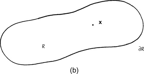
.Consider the configuration of body B![]() at time t, called the present configuration, in which B
at time t, called the present configuration, in which B![]() occupies an open volume R
occupies an open volume R![]() of E3
of E3![]() bounded by a closed surface ∂R
bounded by a closed surface ∂R![]() ; see Figure 3.1(b). (If, for instance, the body B
; see Figure 3.1(b). (If, for instance, the body B![]() is an orange, the region occupied by the flesh constitutes an open volume, and the region occupied the peel constitutes a closed surface.) Let x be the position vector of the place occupied by the representative particle Y at time t; see Figure 3.1(b). Then
is an orange, the region occupied by the flesh constitutes an open volume, and the region occupied the peel constitutes a closed surface.) Let x be the position vector of the place occupied by the representative particle Y at time t; see Figure 3.1(b). Then
x=ˉχ(Y,t).
The mapping (3.1) is called the motion of body B![]() . Note that we distinguish the function ˉχ(Y,t)
. Note that we distinguish the function ˉχ(Y,t)![]() from its value (or output) x. The mapping ˉχ
from its value (or output) x. The mapping ˉχ![]() is assumed to be differentiable as many times as necessary with respect to both Y and t. We also make the important assumption that the motion (3.1) is invertible for each t, so the function exists.
is assumed to be differentiable as many times as necessary with respect to both Y and t. We also make the important assumption that the motion (3.1) is invertible for each t, so the function exists.
Y=ˉχ−1(x,t)
One particular configuration κ of body B![]() may be selected as the reference configuration, and then the body and its motion may be referred to this fixed configuration. A common practice is to choose κ to be the initial configuration, i.e., the configuration occupied by B
may be selected as the reference configuration, and then the body and its motion may be referred to this fixed configuration. A common practice is to choose κ to be the initial configuration, i.e., the configuration occupied by B![]() at time t = 0. However, the reference configuration need not be the initial configuration; in fact, it can even be a configuration that the body B
at time t = 0. However, the reference configuration need not be the initial configuration; in fact, it can even be a configuration that the body B![]() never actually attains. Since the selection of the reference configuration κ is taken from an infinite number of possible configurations of B
never actually attains. Since the selection of the reference configuration κ is taken from an infinite number of possible configurations of B![]() , a motion has infinitely many different referential descriptions, all equally valid.
, a motion has infinitely many different referential descriptions, all equally valid.
In the reference configuration κ, the body B![]() occupies an open volume RR
occupies an open volume RR![]() of E3
of E3![]() bounded by a closed surface ∂RR
bounded by a closed surface ∂RR![]() ; see Figure 3.1(c). Let X be the position vector of the place occupied by the representative particle Y in this reference configuration.The mapping from Y to X is written
; see Figure 3.1(c). Let X be the position vector of the place occupied by the representative particle Y in this reference configuration.The mapping from Y to X is written
X=κ(Y).
The mapping (3.3), called the reference map, is assumed to be differentiable as many times as desired, and invertible. The inverse mapping is
Y=κ−1(X).
Using (3.4), we can rewrite the motion (3.1) as
x=ˉχ[κ−1(X),t]=χκ(X,t).
Equation (3.5) serves as a definition of the mapping κχ. It should be noted that κχ depends on the choice of reference configuration κ. If only one reference configuration is adopted, then the subscript κ is generally omitted, i.e.,
x=χ(X,t),
and the dependence of χ on a particular reference configuration κ is understood.
The function (3.1) is called the material description of motion. In the material description, we deal directly with the particle Y of B![]() . The description of motion (3.6) is called the referential description of motion. In the referential description, the particle Y of B
. The description of motion (3.6) is called the referential description of motion. In the referential description, the particle Y of B![]() is labeled by the position X it occupied when B
is labeled by the position X it occupied when B![]() was in its reference configuration κ.
was in its reference configuration κ.
The displacement u of the particle Y is defined as the difference between its reference and present positions, i.e.,
u=x−X;
see Figure 3.2.

Consider a vector quantity f related to the motion of body B![]() . (Our use of a vector quantity is arbitrary; the discussion that follows is equally valid for a scalar quantity φ or a tensor quantity A.) In the material description, the quantity f is expressed as a function of particle Y and time t, i.e.,
. (Our use of a vector quantity is arbitrary; the discussion that follows is equally valid for a scalar quantity φ or a tensor quantity A.) In the material description, the quantity f is expressed as a function of particle Y and time t, i.e.,
f=ˉf(Y,t).
In the referential description, f is expressed as a function of the position X occupied by Y in the reference configuration κ, and time t. To see this we use (3.4) in (3.8):
f=ˉf(Y,t)=ˉf(κ−1(X),t)=ˆf(X,t).
The quantity f may also be expressed as a function of the position x occupied at time t by the particle Y, and time t. To see this we use (3.2) in (3.8):
f=ˉf(Y,t)=ˉf(ˉχ−1(x,t),t)=ˆf(x,t).
In (3.10) we have expressed f in terms of the present position x of Y, and time t. Such a description is called the spatial description. Referential and spatial descriptions are also referred to as Lagrangian and Eulerian descriptions, respectively.
To review: A vector quantity f (or a scalar quantity φ or a tensor quantity A) related to the motion of body B![]() may be expressed in any of three different descriptions:
may be expressed in any of three different descriptions:
f=ˉf(Y,t)(material)=ˆf(X,t)(referential)=˜f(x,t)(spatial).

This freedom is due to our assumptions that the mappings (3.1) and (3.3) are invertible. In the referential description, each particle is labeled by its reference position; in the spatial description, each particle is labeled by its present position. We note that the material description is seldom used in continuum mechanics since it becomes intractable to find a different name for each particle in the body; the other two representations, however, are useful and will be employed.
Problem 3.1
In a particular motion of body B![]() , the reference configuration is chosen to be the configuration at time t = 0, i.e., the initial configuration. At t = 0, the red particle is at (1, 1, 1), the blue particle is at (0, 0, 0), and the white particle is at (−1, −1, −1). At t = 5 (the present configuration), the red particle is at (2, 2, 2), the blue particle is at (1, 1, 1), and the white particle is at (3, 3, 3), and their temperatures are 5°, 0°, and 10°, respectively; see Figure 3.3.
, the reference configuration is chosen to be the configuration at time t = 0, i.e., the initial configuration. At t = 0, the red particle is at (1, 1, 1), the blue particle is at (0, 0, 0), and the white particle is at (−1, −1, −1). At t = 5 (the present configuration), the red particle is at (2, 2, 2), the blue particle is at (1, 1, 1), and the white particle is at (3, 3, 3), and their temperatures are 5°, 0°, and 10°, respectively; see Figure 3.3.

(a) The equation x=ˉχ(Y,t)![]() answers the question: “Where is particle Y at time t?” That is, the input to the function ˉχ(Y,t)
answers the question: “Where is particle Y at time t?” That is, the input to the function ˉχ(Y,t)![]() is the particle name Y and the time t, and the output is the present position x of the particle at time t. For instance, ˉχ(red,5)=(2,2,2)
is the particle name Y and the time t, and the output is the present position x of the particle at time t. For instance, ˉχ(red,5)=(2,2,2)![]() and ˉχ(blue,5)=(1,1,1)
and ˉχ(blue,5)=(1,1,1)![]() .
.
(b) The equation Y=ˉχ−1(x,t)![]() answers the question: “Which particle is at x at time t?” That is, the input to the function ˉχ−1(x,t)
answers the question: “Which particle is at x at time t?” That is, the input to the function ˉχ−1(x,t)![]() is the time t and the present position x of the particle at time t, and the output is the name Y of the particle. For instance, ˉχ−1((1,1,1),5)=blue
is the time t and the present position x of the particle at time t, and the output is the name Y of the particle. For instance, ˉχ−1((1,1,1),5)=blue![]() .
.
(c) The equation X = κ (Y) answers the question: “Where is particle Y in the reference configuration?” That is, the input to the function κ (Y) is the particle name Y, and the output is the reference position X of the particle. For instance, κ (red) = (1,1,1).
(d) The equation Y = κ−1(X) answers the question: “Which particle is at X in the reference configuration?” That is, the input to the function κ−1(X) is the reference position X of the particle, and the output is the particle name Y. For instance, κ−1(−1, −1, −1) = white.
(e) The equation x = χ (X, t) answers the question: “Where is the particle that was at X in the reference configuration now located at time t?” That is, the input to the function χ (X, t) is the reference position X of the particle and the time t, and the output is the present position x of the particle at time t. For instance, χ ((1,1,1),5) = (2,2,2). To see this, note that
χ((1,1,1),5)=χ(κ(red),5)=ˉχ(red,5)=(2,2,2).
(f) Let Θ be the temperature. The equation Θ=ˉΘ(Y,t)![]() answers the question: “What is the temperature of particle Y at time t?” The input to the function ˉΘ(Y,t)
answers the question: “What is the temperature of particle Y at time t?” The input to the function ˉΘ(Y,t)![]() is the particle name Y and the time t, and the output is the temperature Θ of the particle at time t. For instance, ˉΘ(white,5)=10°
is the particle name Y and the time t, and the output is the temperature Θ of the particle at time t. For instance, ˉΘ(white,5)=10°![]() .
.
(g) The equation Θ=ˆΘ(X,t)![]() answers the question: “What is the temperature at time t of the particle Y that occupied reference position X?” The input to the function ˆΘ(X,t)
answers the question: “What is the temperature at time t of the particle Y that occupied reference position X?” The input to the function ˆΘ(X,t)![]() is the reference position X of the particle and the time t, and the output is the temperature Θ of the particle at time t. For instance, ˆΘ((0,0,0),5)=0°
is the reference position X of the particle and the time t, and the output is the temperature Θ of the particle at time t. For instance, ˆΘ((0,0,0),5)=0°![]() .
.
(h) The equation Θ=˜Θ(x,t)![]() answers the question: “What is the temperature at time t of the particle Y that occupies present position x at time t?” The input to the function ˜Θ(x,t)
answers the question: “What is the temperature at time t of the particle Y that occupies present position x at time t?” The input to the function ˜Θ(x,t)![]() is the time t and the present position x of the particle at time t, and the output is the temperature Θ of the particle at time t. For instance, ˜Θ((2,2,2),5)=5°
is the time t and the present position x of the particle at time t, and the output is the temperature Θ of the particle at time t. For instance, ˜Θ((2,2,2),5)=5°![]() .
.
(i) Note that the material form ˉΘ(Y,t)![]() , the referential form ˆΘ(X,t)
, the referential form ˆΘ(X,t)![]() , and the spatial form ˜Θ(x,t)
, and the spatial form ˜Θ(x,t)![]() are different functions. To illustrate this, note that ˆΘ((1,1,1),5)=5°
are different functions. To illustrate this, note that ˆΘ((1,1,1),5)=5°![]() but ˜Θ((1,1,1),5)=0°
but ˜Θ((1,1,1),5)=0°![]() , i.e., different functions generally provide different output when given identical input.
, i.e., different functions generally provide different output when given identical input.
3.2 Material derivative, velocity, acceleration
Consider once again a vector quantity f related to the motion of body B![]() . The material derivative of f, denoted by ˙f
. The material derivative of f, denoted by ˙f![]() , is defined as the partial derivative of the material description (3.8) of f with respect to time t, holding the label Y fixed:
, is defined as the partial derivative of the material description (3.8) of f with respect to time t, holding the label Y fixed:
˙f=∂∂tˉf(Y,t).
The quantity ˙f![]() can be described as the time rate change of f following a particle. It follows that the velocity v and acceleration a of the particle Y are defined by
can be described as the time rate change of f following a particle. It follows that the velocity v and acceleration a of the particle Y are defined by
v=˙x=∂∂tˉχ(Y,t),a=˙v=∂∂tˉv(Y,t)=∂2∂t2ˉχ(Y,t).
We now determine the referential and spatial descriptions of the material derivative ˙f![]() , which was defined in its impractical material description in (3.11). Using (3.3), (3.9), (3.11), and the chain rule (2.95), we have
, which was defined in its impractical material description in (3.11). Using (3.3), (3.9), (3.11), and the chain rule (2.95), we have
˙f=∂∂tˉf(Y,t)=∂∂tˆf(X,t)+∂∂Xˆf(X,t)∂X∂t=∂∂tˆf(X,t)+∂∂Xˆf(X,t)∂∂tκ(Y)=∂∂tˆf(X,t).

Therefore, in the referential description, ˙f![]() is
is
˙f=∂∂tˆf(X,t),

so the referential forms of the velocity v and acceleration a are
v=˙x=∂∂tχ(X,t),a=˙v=∂∂tˆv(X,t)=∂2∂t2χ(X,t).

These forms give the velocity and acceleration at time t of a particle Y that occupied position X in the reference configuration.
To obtain the spatial description of ˙f![]() , we use (3.1), (3.10), (3.11), (3.12), and the chain rule (2.95):
, we use (3.1), (3.10), (3.11), (3.12), and the chain rule (2.95):
˙f=∂∂tˉf(Y,t)=∂∂t˜f(x,t)+∂∂x˜f(x,t)∂x∂t=∂∂t˜f(x,t)+∂∂x˜f(x,t)∂∂tˉχ(Y,t)=∂∂t˜f(x,t)+∂∂x˜f(x,t)v.

Therefore, the spatial description of ˙f![]() is
is
˙f=∂∂t˜f(x,t)+∂∂x˜f(x,t)v,
so the spatial form of the acceleration a is
a=˙v=∂∂t˜v(x,t)+∂∂x˜v(x,t)v.

This form gives the acceleration at time t of a particle Y that occupies position x at time t.
Similarly, for a scalar quantity φ, we have material, referential, and spatial descriptions of the material derivative:
˙φ=∂∂tˉφ(Y,t),˙φ=∂∂tˆφ(X,t),˙φ=∂∂t˜φ(x,t)+∂∂x˜φ(x,t)·v,

and, for a tensor quantity A,
˙A=∂∂tˉA(Y,t),˙A=∂∂tˆA(X,t),˙A=∂∂t˜A(x,t)+∂∂x˜A(x,t)v.

For a scalar-, vector-, or tensor-valued function of position and time associated with the motion of body B![]() , there are four possible partial derivatives, depending on if the function is considered in its referential form or its spatial form:
, there are four possible partial derivatives, depending on if the function is considered in its referential form or its spatial form:
˙φ=∂∂tˆφ(X,t),φ′=∂∂t˜φ(x,t),Gradφ=∂∂Xˆφ(X,t),gradφ=∂∂x˜φ(x,t),˙f=∂∂tˆf(X,t),f′=∂∂t˜f(x,t),Gradf=∂∂Xˆf(X,t),gradf=∂∂x˜f(x,t),˙A=∂∂tˆA(X,t),A′=∂∂t˜A(x,t),GradA=∂∂XˆA(X,t),gradA=∂∂x˜A(x,t).

We employ this notation throughout the remainder of the book. In words, ˙f![]() denotes the partial derivative of the referential description of f with respect to time (this is a restatement of (3.13)); f′ denotes the partial derivative of the spatial description of f with respect to time; Grad f denotes the gradient of the referential description of f; and grad f denotes the gradient of the spatial description of f. Also, Div f and div f are the divergence of f when considered in its referential and spatial descriptions, respectively. With use of the notation introduced in (3.19), the spatial forms of ˙φ
denotes the partial derivative of the referential description of f with respect to time (this is a restatement of (3.13)); f′ denotes the partial derivative of the spatial description of f with respect to time; Grad f denotes the gradient of the referential description of f; and grad f denotes the gradient of the spatial description of f. Also, Div f and div f are the divergence of f when considered in its referential and spatial descriptions, respectively. With use of the notation introduced in (3.19), the spatial forms of ˙φ![]() , ˙f
, ˙f![]() , and ˙A
, and ˙A![]() (refer to (3.15), (3.17)3, and (3.18)3) become
(refer to (3.15), (3.17)3, and (3.18)3) become
˙φ=φ′+gradφ·v,˙f=f′+(gradf)v,˙A=A′+(gradA)v.
Note that to relate the operations Grad and grad, we have, for instance,
Gradφ=FTgradφ,Gradf=(gradf)F,
where F = Grad x = ∂x/∂X is called the deformation gradient (there is more on this in Section 3.3).
The following forms of the product rule can be verified:
·¯φf=˙φf+φ˙f,·¯f·g=˙f·g+f·˙g,·¯f×g=˙f×g+f×˙g,·¯Af=˙Af+A˙f,·¯AB=˙AB+A˙B,·¯A·B=˙A·B+A·˙B,

where φ is a scalar, f and g are vectors, and A and B are tensors. We also have
·¯A+B=˙A+˙B,·¯AT=(˙A)T.
Problem 3.2
Consider a motion x = χ (X, t) whose Cartesian components are
x1=etX1,x2=e−2tX2,x3=(1+t)X3.
(a) Invert the motion to obtain X = χ−1 (x, t).
(b) Calculate the referential and spatial forms of the displacement u.
(c) Determine the referential and spatial forms of the velocity v.
(d) Calculate the referential and spatial forms of the acceleration a.
(a) Upon inverting the motion x = χ (X, t), we obtain
X1=e−tx1,X2=e2tx2,X3=x31+t.
(b) Recall that the displacement is defined in (3.7); in Cartesian component form, we have
u1=x1−X1,u2=x2−X2,u3=x3−X3.
It follows that the referential form of the displacement is
ˆu1=x1−X1=etX1−X1=(et−1)X1,ˆu2=x2−X2=e−2tX2−X2=(e−2t−1)X2,ˆu3=x3−X3=(1+t)X3−X3=tX3,

while the spatial form is
˜u1=x1−X1=x1−e−tx1=(1−e−t)x1,˜u2=x2−X2=x2−e2tx2=(1−e2t)x2,˜u3=x3−X3=x3−x31+t=t1+tx3.

(c) The referential form of the velocity ˆv(X,t)![]() is obtained using (3.14)1:
is obtained using (3.14)1:
ˆv1=∂x1(X1,X2,X3,t)∂t=∂∂t(etX1)=etX1,ˆv2=∂x2(X1,X2,X3,t)∂t=∂∂t(e−2tX2)=−2e−2tX2,ˆv3=∂x3(X1,X2,X3,t)∂t=∂∂t[(1+t)X3]=X3.

The spatial form of the velocity ˜v(x,t)![]() is obtained by substituting the inverted motion
is obtained by substituting the inverted motion
X1=e−tx1,X2=e2tx2,X3=x31+t
into ˆv1![]() , ˆv2
, ˆv2![]() , and ˆv3
, and ˆv3![]() , yielding
, yielding
˜v1=etX1=et(e−tx1)=x1,˜v2=−2e−2tX2=−2e−2t(e2tx2)=−2x2,˜v3=X3=x31+t.

(d) The referential form of the acceleration ˆa(X,t)![]() is deduced using (3.14)2:
is deduced using (3.14)2:
ˆa1=∂ˆv1(X1,X2,X3,t)∂t=∂∂t(etX1)=etX1,ˆa2=∂ˆv2(X1,X2,X3,t)∂t=∂∂t(−2e−2tX2)=4e−2tX2,ˆa3=∂ˆv3(X1,X2,X3,t)∂t=∂∂t(X3)=0.

The spatial form of the acceleration ˜a(x,t)![]() can be obtained by substituting the inverted motion into ˆa1
can be obtained by substituting the inverted motion into ˆa1![]() , ˆa2
, ˆa2![]() , and ˆa3
, and ˆa3![]() :
:
˜a1=etX1=et(e−tx1)=x1,˜a2=4e−2tX2=4e−2t(e2tx2)=4x2,˜a3=0.

Alternatively, the spatial form of the acceleration ˜a(x,t)![]() can be found using (3.16), whose Cartesian component form is
can be found using (3.16), whose Cartesian component form is
˜ai=∂˜vi(x,t)∂t+∂˜vi(x,t)∂xj˜vj(x,t).

Then,
˜a1=∂˜v1∂t+∂˜v1∂x1˜v1+∂˜v1∂x2˜v2+∂˜v1∂x3˜v3=0+(1)(x1)+0+0=x1,˜a2=∂˜v2∂t+∂˜v2∂x1˜v1+∂˜v2∂x2˜v2+∂˜v2∂x3˜v3=0+0+(−2)(−2x2)+0=4x2,˜a3=∂˜v3∂t+∂˜v3∂x1˜v1+∂˜v3∂x2˜v2+∂˜v3∂x3˜v3=−x3(1+t)2+0+0+x3(1+t)2=0.

Exercises
1. In Cartesian component notation, verify the following forms of the product rule:
(b) ·¯f·g=˙f·g+f·˙g![]() .
.
(c) ·¯f×g=˙f×g+f×˙g![]() .
.
(d) ·¯Af=˙Af+A˙f![]() .
.
(e) ·¯AB=˙AB+A˙B![]() .
.
(f) ·¯A·B=˙A·B+A·˙B![]() .
.
2. In Cartesian component notation, verify that ·¯A+B=˙A+˙B![]() .
.
3. Prove in direct notation that ·¯AT=(˙A)T![]() .
.
3.3 Deformation and strain
A fundamental postulate of classical continuum mechanics is that the response at a particle of the continuum to a deformation at a particular time depends only on the deformation of a small neighborhood of the particle up to that time. We will therefore devote a sizeable amount of space to (1) defining what is meant by the small neighborhood of a particle, (2) defining what is meat by deformation, and (3) describing the kinematical quantities that characterize deformation.
3.3.1 Deformation gradient
The small neighborhood of a particle Y consists of particle Y and all of its nearest neighbors. Suppose Y occupies position X in the reference configuration RR![]() and position x in the present configuration R
and position x in the present configuration R![]() ; refer to Figure 3.1. A vector dX is a filament of infinitesimal length dS in the reference configuration, radiating from X in the direction along unit vector N:
; refer to Figure 3.1. A vector dX is a filament of infinitesimal length dS in the reference configuration, radiating from X in the direction along unit vector N:
dX=NdS.
The line element dX connects particle Y to one of its nearest neighbors in the reference configuration; see Figure 3.4. The small neighborhood of particle Y in the reference configuration RR![]() is the set of all dXs radiating from position X.
is the set of all dXs radiating from position X.

The motion x = χ (X, t) is defined for all particles in the body, i.e., for all X in RR![]() . During this motion, the line element dX will be deformed—in general stretched (or compressed) and rotated, but not bent (dX is too short to be bent)—into a line element dx of length ds, radiating from the new position x of particle Y in the direction along unit vector n:
. During this motion, the line element dX will be deformed—in general stretched (or compressed) and rotated, but not bent (dX is too short to be bent)—into a line element dx of length ds, radiating from the new position x of particle Y in the direction along unit vector n:
dx=nds;
see Figure 3.4. Recall from Section 3.1 that the motion x = χ (X, t) of the body maps each particle Y from its reference position X to its present position x. Since the motion is defined for all particles in the body, the deformation, or change in local geometry, of the small neighborhood of particle Y can be found by evaluating the function χ (X, t) on the particle and all of its nearest neighbors. However, a more tractable approach to quantifying the deformation of this small neighborhood involves defining a deformation measure that can be evaluated at Y alone, so the need to track the motion of all of the nearest neighbors of Y is obviated. This is accomplished through the use of a Taylor series.
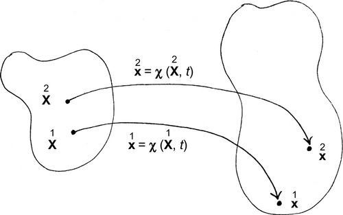
A Taylor series is a mathematical tool that expresses the value of a function at one point in terms of the value of the function and its derivatives at another point. Suppose two particles that occupy points 1X![]() and 2X
and 2X![]() in the reference configuration are mapped to points 1x
in the reference configuration are mapped to points 1x![]() and 2x
and 2x![]() in the present configuration (see Figure 3.5). A Taylor series expansion at 1X
in the present configuration (see Figure 3.5). A Taylor series expansion at 1X![]() gives
gives
2x=χ(2X,t)=χ(1X,t)+[∂χ∂X(1X,t)](2X−1X)+12[∂2χ∂X2(1X,t)](2X−1X)⊗(2X−1X)+…
If 1X![]() and 2X
and 2X![]() are nearest neighbors, then the higher-order terms are negligible, leaving
are nearest neighbors, then the higher-order terms are negligible, leaving
2x=1x+[∂χ∂X(1X,t)](2X−1X).
Upon replacing 1X![]() with X, 2X−1X
with X, 2X−1X![]() with dX, and 2x−1x
with dX, and 2x−1x![]() with dx, we have
with dx, we have
dx=[∂χ∂X(X,t)]dX.
We label
F≡∂χ(X,t)∂X=Gradχ=Gradx,

so
dx=FdX,
where F is called the deformation gradient.
 and 2X
 to their present positions 1x
 and 2x
 .
.Using definition (3.28), one can verify that F satisfies requirements (2.7) and is thus a tensor. Hence, F linearly maps each line element dX radiating from X in the reference configuration into a line element dx radiating from x in the present configuration. (dX is not bent when it is mapped by F to dx.) Therefore F describes the mapping of the small neighborhood of X to the small neighborhood of x, and thus quantifies the changes in the relative positions of nearest neighbors in the body; see Figure 3.6. In other words, F, a function evaluated only at the point X, is a measure of the deformation, or change of local geometry, in the neighborhood of X as it moves to x.
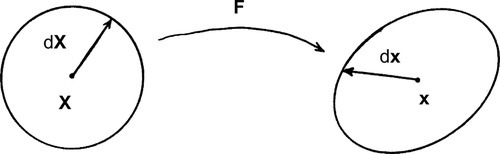
Since F is a linear map, if the small neighborhood of X in the reference configuration is a sphere, then the deformation maps it into an ellipsoid in the present configuration; see Figure 3.6. (If a spherical volume in the reference configuration deforms into a shape other than an ellipsoid, then it is too large to qualify as a small neighborhood, thereby invalidating our truncation of the series (3.26).) Note that although F is a tensor, which is by definition a linear map, the deformation is not restricted to be “linear,” in the sense of infinitesimal. The stretch and rotation of the map from dX to dx can be large.
The tensor F, in general, is a function of position and time, i.e.,
F=ˆF(X,t)=˜F(x,t).
If F is independent of position, i.e., F = F(t), the deformation is said to be homogeneous. If F is independent of time, i.e., F=ˆF(X)=˜F(x)![]() , the deformation is said to be static.
, the deformation is said to be static.
Exercises
1. Prove that the deformation gradient F is a tensor.
3.3.2 Stretch, rotation, green's deformation tensor, cauchy deformation tensor
The deformation gradient F contains the knowledge of what happens, both stretch and rotation, to all elements dX radiating from X in the reference configuration, as they deform to dx in the present configuration at time t. It is worthwhile separating the two concepts of stretch and rotation, which are combined in F, since, as we shall see in later sections, sometimes only one or the other is physically important. We now produce functions of F that isolate stretch or rotation. We will also identify particular elements dX and dx, of the infinitely many radiating from X and x, which have special significance in understanding the deformation.
In general, the line element dX undergoes both stretch and rotation in the deformation (3.28). The ratio
dsdS=λ
of the length of dx to the length of dX is called the stretch λ of the line element. Note that λ is always positive and
λ>1⇒the line element lengthens,λ<1⇒the line element shortens,λ=1⇒the length of the line element remains the same.

Suppose we are interested only in the stretch, and not the rotation, that will happen to a particular line element dX along direction N. Using (3.24) and (3.25), we can rewrite (3.28) as
nds=FNdS,
or, using the definition of stretch (3.30),
λn=FN.
By taking the inner product of (3.32) with itself, we can show that (refer to Problem 3.3)
λ2=N·CN=C·(N⊗N),
where
C=FTF
is called Green's deformation tensor (or the right Cauchy-Green deformation tensor). It can be shown (refer to Problem 3.4) that C is symmetric and positive definite. From relation (3.33), we see that C contains information about the stretch, and not the rotation, that will happen to a line element dX along direction N in the reference configuration.
Problem 3.3
Prove in direct notation that λ2 = N · CN = C · (N ⊗ N).
Upon taking the inner product of (3.32) with itself, we have
λ2n·n=FN·FN.
Since n is a unit vector, n · n = 1. It follows that
λ2=N·FT(FN)=N·(FTF)N,
where we have used definitions (2.11) and (2.13). Thus, since C = FTF,
λ2=N·CN.
Result (2.43) then implies that
λ2=C·(N⊗N).
Problem 3.4
In direct notation, prove that the right Cauchy-Green deformation tensor C is symmetric and positive definite.
We have
CT=(FTF)T=FTFTT=FTF=C,
so, according to definition (2.15), C is symmetric. It follows from (3.33) and positivity of λ that
N·CN>0,
with the unit vector N arbitrary and nonzero, so by (2.53) C is positive definite.
Suppose instead we are interested only in the stretch, and not the rotation, that has happened to a particular dx along direction n in the present configuration. Recall that we assumed in Section 3.1 that the motion x=ˉχ(Y,t)![]() is invertible for all particles Y and times t. Then, using (3.2) and (3.3), we obtain
is invertible for all particles Y and times t. Then, using (3.2) and (3.3), we obtain
X=κ(Y)=κ(ˉχ−1(x,t))=χ−1(x,t),
so the motion x = χ (X, t) is invertible. From linear algebra, it follows that
J≡detF=det(∂x∂X)≠0.

We refer to J ≡ det F as the Jacobian of the deformation gradient, which, as we will see later, is related to the local dilatation or volume change. Inequality (3.36) implies that the tensor F−1 exists, i.e., F = Grad x is invertible:
dX=F−1dx.
Using (3.24) and (3.25), we can rewrite (3.37) as
NdS=F−1nds,
or
1λN=F−1n.
By taking the inner product of (3.38) with itself, we can show that
1λ2=n·cn=c·(n⊗n),
where
c=F−TF−1
is called the Cauchy deformation tensor. It can be verified that c is symmetric and positive definite. From relation (3.39), we see that c contains information about the stretch, and not the rotation, that has happened to a line element dx along direction n in the present configuration.
Therefore, in summary, to find the stretch of a line element without concern for its rotation, if one has knowledge of the shape of the reference configuration (e.g., a specimen in a tensile test), use (3.33), and if one has knowledge of the shape of the deformed configuration (e.g., an inflated inner tube or beach ball), use (3.39).
Exercises
1. Prove in direct notation that 1λ2=n·cn=c·(n⊗n)![]() .
.
2. Prove in direct notation that the Cauchy deformation tensor c is symmetric and positive definite.
3.3.3 Polar decomposition, stretch tensors, rotation tensor
We return to our discussion of the deformation gradient F. Since F is invertible (see (3.37)), it can be decomposed using the polar decomposition theorem (refer to Section 2.3) into the form
F=RU
or
F=VR,
where R is an orthogonal tensor (it will be shown in Sections 3.6 and 4.12 that det F > 0, so R is in fact proper orthogonal), and U and V are symmetric, positive-definite tensors. For physical reasons to be revealed shortly, the tensors R, U, and V are called the rotation tensor, right stretch tensor, and left stretch tensor, respectively.
The effect of the multiplicative decompositions (3.41a) and (3.41b) is to replace the linear transformation (3.28) by either of two pairs of linear transformations:
dx=FdX=(RU)dX=R(UdX),
i.e.,
dX*=UdXfollowed bydx=RdX*,
or
dx=FdX=(VR)dX=V(RdX),
i.e.,
dX*=RdXfollowed bydx=Vdx*;
see Figure 3.7. We emphasize that (3.42a) and (3.42b) involve sequential (or serial) mappings, a distinguishing feature of multiplicative decompositions. Physically, it can be shown that (3.42a) represents stretch followed by pure rotation (refer to Problem 3.6), while (3.42b) represents pure rotation followed by stretch (refer to Problem 3.7).

Problem 3.5
Prove in direct notation that C = U2.
From definition (3.34) and the polar decomposition (3.41a), we have
C=FTF=(RU)T(RU).
It follows from result (2.14)2 that
C=UTRTRU.
Recall that the rotation tensor R is orthogonal, so RTR = I (refer to (2.51)). It follows that
C=UTIU=UTU=UU≡U2
since U is symmetric.
Problem 3.6
Prove in direct notation that decomposition (3.42a) represents stretch followed by pure rotation. That is, show that the deformation (3.42a)1 of dX into dX* involves stretching (and perhaps rotation), and the deformation (3.42a)2 of dX* into dx is rotation without stretch (i.e., pure rotation).
To prove this, we demonstrate that the intermediate element dX* has the same length ds as the deformed element dx; this, in turn, implies that the part of the deformation (3.42a) described by the map U contains all of the stretch of the total deformation from dX to dx, so the part of the deformation (3.42a) described by the map R is pure rotation. To begin, we have
|dX*|2=dX*·dX*=UdX·UdX.
Using definitions (2.11) and (2.13), and noting that U is symmetric, we find that
|dX*|2=dX·UT(UdX)=dX·(UTU)dX=dX·U2dX.
It follows that
|dX*|2=N·U2NdS2=N·CNdS2=λ2dS2=(λdS)2=ds2,
where we have used (3.24), (3.30), (3.33), and C = U2 (refer to Problem 3.5). We then conclude that
|dX*|=|dx|=ds.
Problem 3.7
Prove in direct notation that decomposition (3.42b) represents pure rotation followed by stretch. That is, show that the deformation (3.42b)1 of dX into dx* is pure rotation (rotation without stretch), and the deformation (3.42b)2 of dx* into dx involves stretching (and perhaps rotation).
To prove this, we demonstrate that the intermediate element dx* has the same length dS as the undeformed element dX; this, in turn, implies that the part of the deformation (3.42b) described by the map R is only rotation, and all of the stretch of the total deformation from dX to dx is contained in the map V. To begin, we have
|dx*|2=dx*·dx*=RdX·RdX.
Since R is orthogonal, it follows from definition (2.50) that
|dx*|2=RdX·RdX=dX·dX=|dX|2,
so
|dx*|=|dX|=dS.
3.3.4 Principal stretches and principal directions
Recall the sequential mappings (3.42a) and (3.42b) that arise as a result of the polar decomposition of F, and refer to Figure 3.7. We showed in Problems 3.6 and 3.7 that the maps dx* = R dX and dx = R dX* are pure rotations since they involve no length change. The maps dX* = U dX and dx = V dx*, on the other hand, are called stretches since they incorporate all of the length change of the line element, from length dS of dX to length ds = λdS of dx. In general, these latter two maps also involve a change of direction (or rotation), in addition to this stretch.
When dX is in certain directions, however, the deformation (3.42a)1 from dX to dX* = U dX is pure stretch, i.e., dX* is parallel to dX. Similarly, when dx* = R dX is in certain directions, the deformation (3.42b)2 from dx* to dx = V dx* is pure stretch, i.e., dx is parallel to dx*.
3.3.4.1 Directions of pure stretch in the map U
Recall the map dX* = U dX, where U is the right stretch tensor. The condition that a particular element d1X![]() along direction 1N
along direction 1N![]() undergoes pure stretch in the map U is
undergoes pure stretch in the map U is
d1X*=Ud1X=1λd1X,
or, equivalently,
U1N=1λ1N.
Therefore, if d1X![]() is along a direction 1N
is along a direction 1N![]() that undergoes pure stretch in the map U, then it is along an eigenvector of U, in which case the direction 1N
that undergoes pure stretch in the map U, then it is along an eigenvector of U, in which case the direction 1N![]() is an eigenvector of U, and the stretch 1λ
is an eigenvector of U, and the stretch 1λ![]() that d1X
that d1X![]() undergoes is an eigenvalue of U (refer to Section 2.3).
undergoes is an eigenvalue of U (refer to Section 2.3).
Since U is symmetric and positive definite, there always exist at least three mutually perpendicular eigenvectors 1N![]() , 2N
, 2N![]() , 3N
, 3N![]() of U, with corresponding positive eigenvalues 1λ
of U, with corresponding positive eigenvalues 1λ![]() , 2λ
, 2λ![]() , 3λ
, 3λ![]() . Therefore, there exist at least three directions of pure stretch in the map U, which we will label 1N
. Therefore, there exist at least three directions of pure stretch in the map U, which we will label 1N![]() , 2N
, 2N![]() , 3N
, 3N![]() , with corresponding stretches 1λ
, with corresponding stretches 1λ![]() , 2λ
, 2λ![]() , 3λ
, 3λ![]() . We call 1N
. We call 1N![]() , 2N
, 2N![]() , 3N
, 3N![]() the principal directions, and 1λ
the principal directions, and 1λ![]() , 2λ
, 2λ![]() , 3λ
, 3λ![]() the principal stretches. These three mutually perpendicular unit vectors 1N
the principal stretches. These three mutually perpendicular unit vectors 1N![]() , 2N
, 2N![]() , 3N
, 3N![]() in the directions of pure stretch form an orthonormal basis. With respect to this basis, the matrix of tensor U is diagonal, with components equal to the principal stretches:
in the directions of pure stretch form an orthonormal basis. With respect to this basis, the matrix of tensor U is diagonal, with components equal to the principal stretches:
U=1λ1N⊗1N+2λ2N⊗2N+3λ3N⊗3N=3∑i=1iλiN⊗iN.
Again, refer to Section 2.3.
With this understanding of the principal directions (directions of pure stretch) and principal stretches of U, we can now give the following description of the deformation dx = FdX, as decomposed into dx = R(UdX):
Suppose the small neighborhood of X is a sphere of radius dS. The deformation F takes this sphere into an ellipsoid (see Figure 3.6). In the decomposition F = RU, the sphere is first stretched into an ellipsoid; in this deformation there are (at least) three line elements d1X![]() , d2X
, d2X![]() , d3X
, d3X![]() become the principal axes 1λd1X
become the principal axes 1λd1X![]() , 2λd2X
, 2λd2X![]() , 3λd3X
, 3λd3X![]() of the ellipsoid (see Figure 3.8). The rotation R then rigidly rotates this ellipsoid, so 1N
of the ellipsoid (see Figure 3.8). The rotation R then rigidly rotates this ellipsoid, so 1N![]() (the direction of d1X
(the direction of d1X ![]() ) rotates to 1n
) rotates to 1n![]() , 2N
, 2N![]() rotates to 2n
rotates to 2n![]() , and 3N
, and 3N ![]() rotates to 3n
rotates to 3n ![]() . Since R is a rigid rotation, 1n
. Since R is a rigid rotation, 1n![]() , 2n
, 2n![]() , 3n
, 3n![]() is an orthonormal basis for E3
is an orthonormal basis for E3 ![]() . Therefore,
. Therefore,
R=1n⊗1N+2n⊗2N+3n⊗3N=3∑i=1in⊗iN.
The final product of the composition of these two maps is an ellipsoid with principal axes
d1x=1λ1ndS,d2x=2λ2ndS,d3x=3λ3ndS.
3.3.4.2 Directions of pure stretch in the map V
Suppose d1X![]() is along a direction of pure stretch in U, i.e., d1X
is along a direction of pure stretch in U, i.e., d1X![]() is along an eigenvector of U. Then,
is along an eigenvector of U. Then,
d1x=Fd1X=R(Ud1X)=R(1λd1X)=1λ(Rd1X).
We also have
d1x=Fd1X=V(Rd1X).
Thus,
V(Rd1X)=1λ(Rd1X),
so d1x*=Rd1X![]() is along an eigenvector of the left stretch tensor V. As such, the deformation V takes Rd1X
is along an eigenvector of the left stretch tensor V. As such, the deformation V takes Rd1X![]() to 1λRd1X
to 1λRd1X![]() , so it stretches without rotating. Therefore, the rotation R rotates the principal stretch directions 1N
, so it stretches without rotating. Therefore, the rotation R rotates the principal stretch directions 1N![]() , 2N
, 2N![]() , 3N
, 3N![]() of U into the principal stretch directions 1n
of U into the principal stretch directions 1n![]() , 2n
, 2n![]() , 3n
, 3n![]() of V; see Figure 3.8. Furthermore, the principal stretches 1λ
of V; see Figure 3.8. Furthermore, the principal stretches 1λ![]() , 2λ
, 2λ![]() , 3λ
, 3λ![]() of V are the principal stretches 1λ
of V are the principal stretches 1λ![]() , 2λ
, 2λ![]() , 3λ
, 3λ![]() of U. Hence, V can be expressed as
of U. Hence, V can be expressed as
V=1λ1n⊗1n+2λ2n⊗2n+3λ3n⊗3n=3∑i=1iλin⊗in.

We can now give the following description of the deformation dx = F dX, as decomposed into dx = V(R dX):
Suppose the small neighborhood of X is a sphere of radius dS. The deformation F takes this sphere into an ellipsoid (see Figure 3.6). In the decomposition F = VR, the sphere is first rotated rigidly, and is then stretched into the final ellipsoid. The initial rotation is such that the final stretch is accomplished without any change of direction in the principal axes of the ellipsoid; see Figure 3.8.
Note that R is a rigid rotation of the small neighborhood of X, not of the body as a whole; R can be a function of position, so different parts of the body rotate different amounts.
3.3.5 Other measures of deformation and strain
Recall Green's deformation tensor
C=FTF
and the Cauchy deformation tensor
c=F−TF−1,
which were defined in Section 3.3.2. Also recall that
C=FTF=(RU)T(RU)=UTRTRU=UTIU=UTU=UU≡U2.
We now define
B=FFT,
called the Finger deformation tensor (or the left Cauchy-Green deformation tensor). It can be shown that
B=VV≡V2.
Also, we can verify that
cB=Bc=I,
so
B=c−1.
Suppose 1N![]() is an eigenvector of U, with corresponding eigenvalue 1λ
is an eigenvector of U, with corresponding eigenvalue 1λ![]() . Then
. Then
C1N=UU1N=U(1λ1N)=1λU1N=(1λ)21N.
Therefore, the eigenvectors of C are the eigenvectors of U, and the eigenvalues of C are the squares of the principal stretches. It follows that
C=(1λ)21N⊗1N+(2λ)22N⊗2N+(3λ)23N⊗3N=3∑i=1(iλ)2iN⊗iN.
Similarly, it can be shown that V and B have the same eigenvectors 1n![]() , 2n
, 2n![]() , 3n
, 3n![]() , and that the eigenvalues of B are the squares of the principal stretches, so
, and that the eigenvalues of B are the squares of the principal stretches, so
B=(1λ)21n⊗1n+(2λ)22n⊗2n+(3λ)23n⊗3n=3∑i=1(iλ)2in⊗in.
All of the measures of deformation we have so far defined, namely, F, F−1, C, c, B, R, U, and V, reduce to the identity tensor in the absence of deformation:
x=X⇒F=F−1=C=c=B=R=U=V=I.
We now define two additional measures,
E=12(C−I),
called the Lagrangian strain tensor (or Green-Lagrange strain tensor), and
e=12(I−c),
called the Eulerian strain tensor (or Euler-Almansi strain tensor). These strain tensors vanish in the absence of deformation:
x=X⇒E=e=0.
Recall that C, c, U, and V are symmetric; it can be shown that B, E, and e are also symmetric.
The deformation and strain tensors presented heretofore can be expressed in terms of the displacement u = x − X. For instance, we have
C=(Gradx)TGradx=[Grad(X+u)]TGrad(X+u)=(I+Gradu)T(I+Gradu)=I+Gradu+(Gradu)T+(Gradu)TGradu

and
E=12(C−I)=12[Gradu+(Gradu)T+(Gradu)TGradu].
Similarly,
c=I−gradu−(gradu)T+(gradu)Tgradu
and
e=12(I−c)=12[gradu+(gradu)T−(gradu)Tgradu].
Equations (3.54) and (3.55) are referred to as strain-displacement relations.
Problem 3.8
Given the motion
x1=−2X1+X2,x2=−X1−2X2,x3=X3,
determine matrix representations of
(a) the deformation gradient F, Green's deformation tensor C, the Finger deformation tensor B, and the Cauchy deformation tensor c;
(b) the Lagrangian strain tensor E and the Eulerian strain tensor e;
(c) the right stretch tensor U, the left stretch tensor V, and the rotation tensor R.
(a) We have x = xiei and X = XAeA, where ei and eA are the Cartesian basis vectors associated with the present and reference configurations, respectively. (Note that lowercase subscripts pertain to the present configuration, and uppercase subscripts pertain to the reference configuration.) It then follows from (3.27) that the Cartesian components of the deformation gradient are FiA = ∂xi/∂XA, which in turn implies that
F=FiAei⊗eA=∂xi∂XAei⊗eA.

Thus, using (2.34), we have
[F]=[∂x1∂X1∂x1∂X2∂x1∂X3∂x2∂X1∂x2∂X2∂x2∂X3∂x3∂X1∂x3∂X2∂x3∂X3]=[−210−1−20001].

Note that the deformation is homogeneous since the components of F are independent of position X, and static since the components of F are independent of time t. Then, since C = FTF, it follows from (2.35) and (2.37) that
[C]=[F]T[F]=[−2−101−20001][−210−1−20001]=[500050001].

Similarly,
[B]=[F][F]T=[−210−1−20001][−2−101−20001]=[500050001],

and
[c]=[F]−T[F]−1=[−25150−15−250001][−25−15015−250001]=[15000150001].

Note that, as expected, [c]−1 = [B].
(b) Recall that E=12(C−I)![]() ; it follows from (2.36) that
; it follows from (2.36) that
[E]=12([C]−[I])=12([500050001]−[100010001])=[200020000].

Similarly,
[e]=12([I]−[c])=12([100010001]−[15000150001])=[25000250000].

(c) To calculate the right stretch tensor U, we use the relationship U2 ≡ UU = C. Since [C] is a diagonal matrix in this example, [U] is obtained by taking the square root of each of the elements of [C], i.e.,
[U]=[√C]=[√5000√50001].

Similarly,
[V]=[√B]=[√5000√50001].

(To calculate the square root of a matrix with nonzero off-diagonal terms, the matrix is first re-expressed in terms of its basis of eigenvectors, which results in a diagonal representation of the matrix. The square root of this diagonal matrix is calculated as shown above, i.e., by taking the square root of the diagonal elements. The resulting matrix is then rotated back to the original Cartesian basis.)
Finally, we use the relationship R = FU−1 to calculate the rotation tensor:
[R]=[F][U]−1=[−210−1−20001][1√50001√50001]=[−2√51√50−1√5−2√50000].
Note that since R is orthogonal,
detR=det[R]=(−2√5)2−(1√5)(−1√5)=1,

as expected.