
Nonlinear Elasticity
Abstract
This chapter presents constitutive equations appropriate for a broad class of engineering materials known as nonlinear elastic solids. Common examples include rubber, elastomers (rubber-like polymers), and soft biological tissues. Nonlinear elastic solids are characterized by their ability to undergo large recoverable deformations and their highly nonlinear stress-strain response. Hence, they exhibit geometric nonlinearity (i.e., strain-displacement nonlinearity) due to finite elastic deformations, and material nonlinearity (i.e., stress-strain nonlinearity) due to nonlinear constitutive response. We examine nonlinear elastic materials in the context of the mechanical (isothermal) theory as well as the thermomechanical theory. In the latter case, we explicitly illustrate how the constitutive equations must satisfy the second law of thermodynamics, invariance, conservation of angular momentum, and material symmetry (isotropy).
This chapter presents constitutive equations appropriate for a broad class of engineering materials known as nonlinear elastic solids. Common examples include rubber, elastomers (rubberlike polymers), and soft biological tissues. Nonlinear elastic solids are characterized by their ability to undergo large deformations before yielding, and their highly nonlinear stress-strain response.1,2 Hence, they exhibit geometric nonlinearity (or strain-displacement nonlinearity) owing to finite elastic deformations, and material nonlinearity owing to nonlinear constitutive response. Sections 6.1 and 6.2 discuss nonlinear elastic materials in the context of the mechanical (isothermal) theory and the thermomechanical theory, respectively. In the latter case, we explicitly illustrate how the constitutive equations must satisfy the second law of thermodynamics, invariance, conservation of angular momentum, and material symmetry (isotropy).
6.1 Mechanical theory
Recall from Section 5.1 that in the Eulerian formulation of the mechanical theory, a constitutive assumption is made on the Cauchy stress T as a function of the motion χ, and possibly its rates, gradients, and history, i.e.,
T=˘T(motion).
For an elastic material, which has a perfect memory of some reference configuration, the Cauchy stress T at position x and time t depends on the motion only through the strain at x and t with respect to the reference configuration. The deformation gradient F = Grad χ (refer to Section 3.3.1) is a measure of this relative strain, so we may write
T=˘T(F).
We emphasize that the stress at position x and time t in an elastic material depends only on the strain at x and t, and neither the history nor the rate of the strain (refer to Appendix B).
Equation (6.1) implies that the stress T at position x and time t is an explicit function of the deformation gradient F = Grad χ with respect to some reference configuration X, evaluated at the same x and t. Therefore, implicit in (6.1) is a dependence of T on a reference configuration X. Also implicit in (6.1) is a dependence of T on x and t, and a possible dependence of T on the present density ρ, since ρ is an algebraic function of the reference density ρR and the deformation gradient F:
ρ=ρRdetF.
At this stage, it is useful to appeal to the mechanical energy balance
ρ˙ε=T·D,
which is the first law of thermodynamics (5.26) specialized to a mechanical setting. Essentially, (6.2) indicates that in the mechanical theory, the rate of change of the internal energy ε is due solely to the stress power T · D; refer to Section 4.7. Arguing that the internal energy ε (like the Cauchy stress T) is a function of the strain F alone, i.e.,
ε=˘ε(F),
and using the results of Problem 6.2 (which appear in the upcoming section), we have
˙ε=d˘εdF·˙F=d˘εdFFT·L.

Hence, the mechanical energy balance (6.2) becomes
(T−ρd˘εdFFT)·L=0,

noting that T · L = T · D (refer to Problem 6.1 in the upcoming section). Since the coefficient of L in (6.3) is independent of L, and L is arbitrary, it follows that
T=ρd˘εdFFT.

That is, the derivative of the internal energy ε with respect to the strain F gives the stress T. Hence, the internal energy is a strain energy. The class of materials for which the stress-strain response is derived from a strain energy potential, or stored elastic energy, is called hyperelastic.
Problem 6.1
In direct notation, show that T · L = T · D.
T·L=T·(D+W)(decomposition(3.57))=T·D+T·W(property(2.6)3)=T·D(result(2.44)).

In the second step, we were able to employ the distributive property (2.6)3 of the inner product since it was demonstrated (in Problem 2.34) that the set of all second-order tensors is an inner product space. In the third step, we have exploited that T · W = 0, since T is symmetric (by conservation of angular momentum; see (5.25)) and W is skew (by construction; see (3.58)2).
Problem 6.2
Prove in direct notation that ∂ψ∂F·˙F=∂ψ∂FFT·L![]() .
.
∂ψ∂F·˙F=∂ψ∂F·(LF)(result(3.60)1)=tr[∂ψ∂F(LF)T](definition(2.41))=tr[∂ψ∂F(FTLT)](result(2.14)2)=tr[(∂ψ∂FFT)LT](associativity of tensor multiplication)=∂ψ∂FFT·L(definition(2.41)).

Recall from Section 5.2 that the constitutive equation (6.4) for the Cauchy stress T must satisfy conservation of angular momentum, invariance requirements, and material symmetry conditions. We postpone the exploration of these requirements until Section 6.2.
6.2 Thermomechanical theory
Recall from Section 5.3 that in formulation (5.36)–(5.38) of the thermomechanical theory, constitutive assumptions are made on the Cauchy stress T, heat flux vector q, Helmholtz free energy ψ, and entropy η as functions of the motion χ and temperature Θ, and possibly their rates, gradients, and histories, i.e.,
T=ˉT(motion and temperature),q=ˉq(motion and temperature),ψ=ˉψ(motion and temperature),η=ˉη(motion and temperature).
For a thermoelastic material, which has a perfect memory of its reference configuration and temperature, the list of arguments in (6.1) is expanded from χ (implicit) and F = Grad χ (explicit) to include the analogous thermal quantities Θ and gR = GradΘ. Therefore, for a thermoelastic material, we write
T=ˉT(F,Θ,gR),q=ˉq(F,Θ,gR),ψ=ˉψ(F,Θ,gR),η=ˉη(F,Θ,gR).
This notation means that T, q, ψ, and η at position x and time t are explicit functions of F, Θ, and gR evaluated at x and t (and, thus, implicit functions of x and t). There is an implicit dependence on the reference configuration X through F = Grad χ and gR = Grad Θ. Recall from (4.65) the relationship gR = FTg between the referential and spatial temperature gradients, so gR is a function of g and F. We may therefore replace (6.5) with
T=˘T(F,Θ,g),q=˘q(F,Θ,g),ψ=˘ψ(F,Θ,g),η=˘η(F,Θ,g).
Note that ˉT![]() in (6.5) and ˘T
in (6.5) and ˘T![]() in (6.6) denote two different response functions for T. Also note that the constitutive functions for T, q, ψ, and η in (6.6) do not depend on the history or the rate of the strain or temperature (refer to Appendix B).
in (6.6) denote two different response functions for T. Also note that the constitutive functions for T, q, ψ, and η in (6.6) do not depend on the history or the rate of the strain or temperature (refer to Appendix B).
Now that a list of arguments has been specified for the constitutive functions that characterize a thermoelastic material, the number of independent constitutive functions, and the list of arguments itself, can be reduced. As described in Section 5.4 and illustrated in the following sections, this reduction is accomplished via the second law of thermodynamics, invariance requirements, conservation of angular momentum, and material symmetry considerations.
6.2.1 Restrictions imposed by the second law of thermodynamics
Substitution of the constitutive assumptions (6.6) into the Clausius-Duhem inequality (5.35) gives
−ρ∂˘ψ∂F·˙F+˘T·D−ρ(∂˘ψ∂Θ+˘η)˙Θ−ρ∂˘ψ∂g·˙g−1Θ˘q·g≥0,

where we have used the chain rule (refer to Section 2.5.2):
˙ψ=∂˘ψ∂F·˙F+∂˘ψ∂Θ˙Θ+∂˘ψ∂g·˙g.

It can be shown (refer to Problems 6.1 and 6.2) that
˘T·D=˘T·L,∂˘ψ∂F·˙F=∂˘ψ∂FFT·L,
so inequality (6.7) becomes
(˘T−ρ∂˘ψ∂FFT)·L−ρ(∂˘ψ∂Θ+˘η)˙Θ−ρ∂˘ψ∂g·˙g−1Θ˘q·g≥0.

Inequality (6.8) must hold for all processes. In particular, it must hold for the family of processes with g = 0, ˙g=0![]() , and L = 0, but ˙Θ
, and L = 0, but ˙Θ![]() arbitrary, at particular position x and time t. (An example is the family of processes (D.1) in Appendix D with A = 0, a = 0, and g0 = 0, but a any real number.) For members of this family of processes, (6.8) simplifies to
arbitrary, at particular position x and time t. (An example is the family of processes (D.1) in Appendix D with A = 0, a = 0, and g0 = 0, but a any real number.) For members of this family of processes, (6.8) simplifies to
−ρ(∂˘ψ∂Θ+˘η)˙Θ≥0.

The density ρ is positive, which implies
(∂˘ψ∂Θ+˘η)˙Θ≥0.

The coefficient of ˙Θ![]() in (6.9) is independent of ˙Θ
in (6.9) is independent of ˙Θ![]() . For (6.9) to hold for all members of this family, the coefficient of ˙Θ
. For (6.9) to hold for all members of this family, the coefficient of ˙Θ![]() must vanish, i.e.,
must vanish, i.e.,
η=−∂˘ψ∂Θ.
Thus, the partial derivative of the response function for the Helmholtz free energy ψ with respect to temperature Θ gives the value of the entropy η, so ˘η![]() is not an independent response function. Result (6.10) holds for all processes, not just the special family considered above. Hence, inequality (6.8) reduces to
is not an independent response function. Result (6.10) holds for all processes, not just the special family considered above. Hence, inequality (6.8) reduces to
(˘T−ρ∂˘ψ∂FFT)·L−ρ∂˘ψ∂g·˙g−1Θ˘q·g≥0.

Inequality (6.11) must hold for all processes, in particular the family of processes with g = 0 and L = 0, but ˙g![]() arbitrary, at x and t (e.g., the family (D.1) in Appendix D with A = 0 and g0 = 0, but a any vector). For members of this family, (6.11) simplifies to
arbitrary, at x and t (e.g., the family (D.1) in Appendix D with A = 0 and g0 = 0, but a any vector). For members of this family, (6.11) simplifies to
−ρ∂˘ψ∂g·˙g≥0.
The density is positive; hence,
∂˘ψ∂g·˙g≤0.

The coefficient of ˙g![]() in (6.12) is independent of ˙g
in (6.12) is independent of ˙g ![]() . Hence, the rate ˙g
. Hence, the rate ˙g![]() may be chosen to violate the inequality (6.12) unless its coefficient is the zero vector. Therefore,
may be chosen to violate the inequality (6.12) unless its coefficient is the zero vector. Therefore,
∂˘ψ∂g=0.
Thus, if the response function for ψ depended on the temperature gradient g, the second law would be violated for some processes. Since the second law must be obeyed for all processes, we conclude that a thermoelastic response function for ψ must be independent of g. Inequality (6.11) thus reduces to
(˘T−ρ∂˘ψ∂FFT)·L−1Θ˘q·g≥0.

which must hold for all processes.
Consider those processes with g = 0 but L arbitrary at x and t (e.g., the family (D.1) in Appendix D with g0 = 0, F0 fixed and invertible, and A any tensor). For these processes, (6.13) simplifies to
(˘T−ρ∂˘ψ∂FFT)·L≥0.
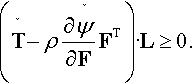
The coefficient of the rate L in (6.14) is independent of rates. Hence, we obtain
T=ρ∂˘ψ∂FFT.

Thus, the partial derivative of the response function for the Helmholtz free energy ψ with respect to strain F gives the value of the stress T, i.e., the Helmholtz free energy is a strain energy. Recall that the class of materials for which the stress-strain response is derived from a strain energy potential is called hyperelastic. The inequality (6.13) thus reduces to
−1Θ˘q·g≥0
or
˘q·g≤0,
since the absolute temperature Θ is strictly positive. Inequality (6.15) cannot be simplified any further since ˘q![]() depends on g. Thus, the Clausius-Duhem inequality has been reduced for thermoelastic materials to an intuitive statement of the second law: heat flows against the temperature gradient, from hot to cold.
depends on g. Thus, the Clausius-Duhem inequality has been reduced for thermoelastic materials to an intuitive statement of the second law: heat flows against the temperature gradient, from hot to cold.
We now pause and take stock of our accomplishments. By demanding that the Clausius-Duhem inequality holds for all thermoelastic processes, we have reduced the constitutive assumption (6.6) to
ψ=˘ψ(F,Θ),q=˘q(F,Θ,g)with˘q·g≤0,
and
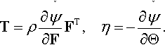
T=ρ∂˘ψ∂FFT,η=−∂˘ψ∂Θ.
Thus, as a consequence of the second law, we have found that:
(1) Only two response functions ( ˘ψ![]() and ˘q
and ˘q![]() ) are needed to characterize a thermoelastic material, rather than the four initially supposed. (Nice! Fewer response functions means fewer unknowns in the characterization problem.)
) are needed to characterize a thermoelastic material, rather than the four initially supposed. (Nice! Fewer response functions means fewer unknowns in the characterization problem.)
(2) The response function for ψ is independent of g. (Again, fewer experiments to perform.)
(3) The response function for q is restricted by the second law through the inequality ˘q·g≤0![]() , i.e., heat flows against the temperature gradient.
, i.e., heat flows against the temperature gradient.
It can be shown (refer to Problem 6.3) that if the heat flux vector ˘q![]() in (6.6) is a continuous function of temperature gradient g at g = 0, restriction (3) above has an additional implication: ˘q
in (6.6) is a continuous function of temperature gradient g at g = 0, restriction (3) above has an additional implication: ˘q![]() evaluated at g = 0 is zero, i.e., heat does not flow in the absence of a temperature gradient.
evaluated at g = 0 is zero, i.e., heat does not flow in the absence of a temperature gradient.
Problem 6.3
Show that if the heat flux vector ˘q![]() in (6.6) is a continuous function of the temperature gradient g at g = 0, then it follows from ˘q·g≤0
in (6.6) is a continuous function of the temperature gradient g at g = 0, then it follows from ˘q·g≤0![]() that ˘q
that ˘q![]() evaluated at g = 0 is zero. That is, heat does not flow in the absence of a temperature gradient.
evaluated at g = 0 is zero. That is, heat does not flow in the absence of a temperature gradient.
If ˘q![]() is a continuous function of g at g = 0, then it follows that
is a continuous function of g at g = 0, then it follows that
q=˘q(F,Θ,g)=a(F,Θ)+b(F,Θ,g),
with
limα→0b(F,Θ,αg)=0,
so
˘q(F,Θ,g)|g=0=limα→0˘q(F,Θ,αg)=a(F,Θ).
Then ˘q·g≤0![]() implies
implies
a(F,Θ)·g+b(F,Θ,g)·g≤0.
Replacing g by αg, taking α > 0, and dividing by α leads to
a(F,Θ)·g+b(F,Θ,αg)·g≤0.
Taking the limit as α → 0 gives
a(F,Θ)·g≤0,
which must hold for all processes. Since a(F, Θ) is independent of g, this implies that a(F, Θ) = 0, or
˘q(F,Θ,g)|g=0=0.
6.2.2 Restrictions imposed by invariance under superposed rigid body motions and conservation of angular momentum
Our appeal to the second law has proven fruitful. We now appeal to invariance requirements under superposed rigid body motions (refer to Sections 5.2.1 and 5.4.1) and obtain further restrictions. (Note that any restrictions on the response functions are very helpful, as they reduce the number of experiments needed to characterize a particular material.) In particular, we must have
ψ+=ψ,q+=Qq
when
F+=QF,Θ+=Θ,g+=Qg
for all proper orthogonal tensors Q(t). It can be shown (refer to Problems 6.4 and 6.5) that these invariance requirements demand
ψ=˘ψ(F,Θ)=′ψ(C,Θ)
and
q=˘q(F,Θ,g)=Fq‵(C,Θ,gR).
Note that ˘ψ![]() and ‵ψ
and ‵ψ![]() denote two different response functions for ψ. Equation (6.17) implies that the response function for ψ can depend on F only through the combination C = FTF, where C is Green's deformation tensor; the dependence on Θ is unrestricted. Equation (6.18) implies that the dependence of the response function for q on g must be through gR = FTg (where gR is the referential temperature gradient), there must be a linear dependence of q on F, and any further dependence on F must be through the combination C = FTF.
denote two different response functions for ψ. Equation (6.17) implies that the response function for ψ can depend on F only through the combination C = FTF, where C is Green's deformation tensor; the dependence on Θ is unrestricted. Equation (6.18) implies that the dependence of the response function for q on g must be through gR = FTg (where gR is the referential temperature gradient), there must be a linear dependence of q on F, and any further dependence on F must be through the combination C = FTF.
Problem 6.4
Prove that the invariance requirement ψ+ = ψ is satisfied if and only if
ψ=˘ψ(F,Θ)=‵ψ(C,Θ).
The phrase “if and only if” requires that we demonstrate both necessity and sufficiency in our proof. To demonstrate necessity, we must show that the invariance requirement ψ+ = ψ implies that ψ=‵ψ(C,Θ)![]() . To demonstrate sufficiency, we must show that ψ=‵ψ(C,Θ)
. To demonstrate sufficiency, we must show that ψ=‵ψ(C,Θ)![]() satisfies the invariance requirement ψ+ = ψ.
satisfies the invariance requirement ψ+ = ψ.
Necessity: First, note that
ψ=˘ψ(F,Θ),ψ+=˘ψ(F+,Θ+).
The invariance requirement
ψ+=ψwhenF+=QF,Θ+=Θ
for all proper orthogonal Q implies that
˘ψ(QF,Θ)=˘ψ(F,Θ).
Since this must hold for all proper orthogonal Q, it must hold for the particular case Q = RT, so
˘ψ(F,Θ)=˘ψ(RTF,Θ).
(Recall from Section 3.3.3 that R is the proper orthogonal rotation tensor in the polar decomposition of F.) Since
RTF=RTRU=IU=U=C1/2.
it follows that
ψ=˘ψ(F,Θ)=˘ψ(RTF,Θ)=˘ψ(U,Θ)=˘ψ(C1/2,Θ)=‵ψ(C,Θ).
Sufficiency: It follows from ψ=‵ψ(C,Θ)![]() that
that
ψ+=‵ψ(C+,Θ+)=‵ψ(C,Θ)=ψ,
where we have used the results C+ = C and Θ+ = Θ from Sections 5.2.1.2 and 5.4.1.1.
Problem 6.5
Prove that the invariance requirement q+ = Qq is satisfied if and only if
q=˘q(F,Θ,g)=F‵q(C,Θ,FTg).
As was the case in Problem 6.4, the phrase “if and only if” requires that we demonstrate both necessity and sufficiency in our proof. To demonstrate necessity, we must show that the invariance requirement q+ = Qq implies that q=F‵q(C,Θ,FTg)![]() . To demonstrate sufficiency, we must show that q=F‵q(C,Θ,FTg)
. To demonstrate sufficiency, we must show that q=F‵q(C,Θ,FTg)![]() satisfies the invariance requirement q+ = Qq.
satisfies the invariance requirement q+ = Qq.
Necessity: First, note that
q=˘q(F,Θ,g),q+=˘q(F+,Θ+,g+).
The invariance requirement
q+=QqwhenF+=QF,Θ+=Θ,g+=Qg
implies that
˘q(QF,Θ,Qg)=Q˘q(F,Θ,g),
which must hold for all proper orthogonal Q, and, in particular, Q = RT. Since
RTF=RTRU=IU=U,
it follows that
˘q(F,Θ,g)=R˘q(U,Θ,RTg).
We define a new function ˉq![]() by
by
˘q(U,Θ,RTg)=Uˉq(U,Θ,URTg),
which gives
˘q(F,Θ,g)=RUˉq(U,Θ,URTg).
We have
F=RU,FT−(RU)T=UTRT=URT,U=C1/2,
which imply that
˘q(F,Θ,g)=Fˉq(C1/2,Θ,FTg)=Fq′(C,Θ,FTg).
Sufficiency: It follows from q=F′q(C,Θ,FTg)![]() that
that
q+=F+′q(C+,Θ+,(F+)Tg+)=QF′q(C,Θ,FTQTQg)=QF′q(C,Θ,FTg)=Qq,

where we have used the results F+ = QF, C+ = C, g+ = Qg, and Θ+ = Θ from Sections 5.2.1.2 and 5.4.1.1.
Now that we have established ψ=‵ψ(C,Θ)![]() , it can be shown, through a change of independent variable from F to C, that (6.16b)1 becomes
, it can be shown, through a change of independent variable from F to C, that (6.16b)1 becomes
T=ρ∂˘ψ(F,Θ)∂FFT=ρF(∂‵ψ(C,Θ)∂C+∂′ψ(C,Θ)∂CT)FT.
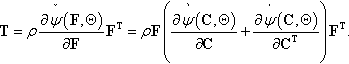
If ‵ψ(C,Θ)![]() is a symmetric function of C, then (6.19) becomes
is a symmetric function of C, then (6.19) becomes
T=2ρF∂‵ψ(C,Θ)∂CFT.
It can be shown that (6.19) and (6.20) ensure that the Cauchy stress T is symmetric, so conservation of angular momentum (5.25) is satisfied.
To summarize the results of this section thus far: A thermoelastic material has a perfect memory of its reference state. On physical grounds, it is assumed that such a material is characterized by at most four response functions, each of which could conceivably depend on the deformation gradient F (with respect to some reference configuration), temperature Θ, and temperature gradient g, all evaluated at present time t (i.e., the response at present time t depends on the present values of F, Θ, and g). The four response functions and their lists of arguments are
T=˘T(F,Θ,g),q=˘q(F,Θ,g),ψ=˘ψ(F,Θ,g),η=˘η(F,Θ,g).
Note that the dependence on deformation does not involve its history, but rather just the present value of the deformation gradient from some reference configuration.
Because these response functions must be consistent with conservation of angular momentum, the second law of thermodynamics for all thermomechanical processes, and invariance requirements under any superposed rigid body motion, we find that only two of the response functions are independent, i.e.,
ψ=‵ψ(C,Θ),q=F‵q(C,Θ,gR),
from which
T=2ρF∂‵ψ(C,Θ)∂CFT,η=−∂‵ψ(C,Θ)∂Θ

can be deduced, with the restrictions
‵q(C,Θ,0)=0,q·g≤0.
Note that the Helmholtz free energy, Cauchy stress, and entropy are independent of temperature gradient. Also note that the Clausius-Duhem inequality reduces to the intuitive second law statements (6.21c)1 and (6.21c)2, i.e., heat does not flow in the absence of a temperature gradient, and in the presence of a temperature gradient, heat flows opposite the temperature gradient, from hot to cold.
Exercises
1. Using indicial notation, verify through a change of independent variable from F to C that
T=ρ∂˘ψ(F,Θ)∂FFT=ρF(∂‵ψ(C,Θ)∂C+∂‵ψ(C,Θ)∂CT)FT=2ρF∂‵ψ(C,Θ)∂CFT,

where the last equality holds if ‵ψ(C,Θ)![]() is a symmetric function of C, i.e.,
is a symmetric function of C, i.e.,
∂′ψ(C,Θ)∂C=∂′ψ(C,Θ)∂CT.
2. Verify that (6.19) and (6.20) ensure that the Cauchy stress T is symmetric, so conservation of angular momentum is satisfied.
6.2.3 Restrictions imposed by material symmetry: isotropy
In this section, we apply material symmetry considerations (refer to Section 5.2.2) to further reduce and simplify the form of the response functions. In particular, we consider thermoelastic materials that are isotropic. Loosely speaking, isotropic materials have properties that are identical in all directions.
Recall from Section 6.2.1 that by demanding the Clausius-Duhem inequality hold for all thermoelastic processes, we found that only two response functions are necessary to characterize a thermoelastic material, i.e.,
ψ=˘ψ(F,Θ),q=˘q(F,Θ,g),
where the dependence of the deformation gradient F on a particular reference configuration κ is understood. Here, κ is chosen to be the stress-free configuration. By analogy to (5.22), we have
˘ψ(F,Θ)=˘ψ(FH−1,Θ)for allH∈G,
where G![]() is the symmetry group of the material relative to the stress-free reference configuration κ, and H is a symmetry transformation with respect to κ. Since a thermoelastic material is a solid, we have G⊆O
is the symmetry group of the material relative to the stress-free reference configuration κ, and H is a symmetry transformation with respect to κ. Since a thermoelastic material is a solid, we have G⊆O![]() , where O
, where O![]() is the full orthogonal group. Then (6.22) becomes
is the full orthogonal group. Then (6.22) becomes
˘ψ(F,Θ)=˘ψ(FHT,Θ)for allH∈G.
Recall from Section 6.2.2 that in order to satisfy invariance under superposed rigid body motions and conservation of angular momentum, we must specify ψ to be a function of F in the particular combination C = FTF, i.e.,
ψ=′ψ(C,Θ),
where C is Green's deformation tensor. The condition on ‵ψ![]() corresponding to (6.23) is
corresponding to (6.23) is
‵ψ(C,Θ)=‵ψ(HCHT,Θ)for allH∈G.
For isotropic thermoelastic solids, the symmetry group G![]() relative to the stress-free reference configuration κ is the full orthogonal group O
relative to the stress-free reference configuration κ is the full orthogonal group O![]() . Therefore, (6.24) becomes
. Therefore, (6.24) becomes
‵ψ(C,Θ)=‵ψ(HCHT,Θ)for allH∈O.
The requirement (6.25) on the functional form of ‵ψ![]() is equivalent to the condition that ‵ψ
is equivalent to the condition that ‵ψ![]() depend on C only through the principal scalar invariants of C, i.e.,
depend on C only through the principal scalar invariants of C, i.e.,
ψ=ˉψ(I1,I2,I3,Θ),
where
I1=trC,I2=12[(trC)2−tr(C2)],I3=detC.
Recalling that the Cauchy stress T is obtained from the Helmholtz free energy ψ by
T=2ρF∂‵ψ(C,Θ)∂CFT,

we have, through a change of independent variable,
T=2ρF(∂ˉψ∂I1dI1dC+∂ˉψ∂I2dI2dC+∂ˉψ∂I3dI3dC)FT.

Recall from Section 2.5.1 the results
dI1dC=I,dI2dC=I1I−C,dI3dC=I3C−1.

Substitution of (6.28) into (6.27) gives
T=α0I+α1B+α2B2,
where B = FFT is the Finger deformation tensor and
α0=2ρI3∂ˉψ∂I3,α1=2ρ(∂ˉψ∂I1+I1∂ˉψ∂I2),α2=−2ρ∂ˉψ∂I2.

Note that since B and C have the same eigenvalues, they also have the same principal invariants (refer to Sections 2.3 and 3.3.5). Use of the Cayley-Hamilton theorem (2.75) gives the alternative form
T=β0I+β1B+β−1B−1,
where
β0=2ρ(I2∂ˉψ∂I2+I3∂ˉψ∂I3),β1=2ρ∂ˉψ∂I1,β−1=−2ρI3∂ˉψ∂I2.

In nonlinear elasticity it is common to speak of the strain energy W per unit reference volume, i.e., the strain energy density, defined by
W=ρRψ,
rather than the Helmholtz free energy. For isotropic thermoelastic materials, we have
W=ˉW(I1,I2,I3,Θ).
It follows that (6.30b) becomes
β0=2I−123(I2∂ˉW∂I2+I3∂ˉW∂I3),β1=2I−1/23∂ˉW∂I1β−1=−2I1/23∂ˉW∂I2,

where we have used
ρρR=1J=1detF=I−1/23,

which follows from conservation of mass (4.56a). Recall that ρ is the density in the present configuration, ρR is the density in the reference configuration, and J is the determinant of the deformation gradient F.
Exercises
1. Verify that substitution of (6.28) into (6.27) gives (6.29a) and (6.29b).
2. Verify that (6.30a) and (6.30b) follow from (6.29a) and (6.29b) and use of the Cayley-Hamilton theorem.
3. Verify (6.31).
6.3 Strain energy models
We found in Section 6.2 that the Cauchy stress for an isotropic nonlinear elastic material can be expressed as
T=β0I+β1B+β−1B−1,
where
β0=2I−1/23(I2∂ˉW∂I2+I3∂ˉW∂I3),β1=2I−1/23∂ˉW∂I1β−1=−2I1/23∂ˉW∂I2,

B = FFT is the Finger deformation tensor, W=ˉW(I1,I2,I3,Θ)![]() is the strain energy density, and I1, I2, and I3 are the principal invariants of B. We now specialize this constitutive model to the mechanical (isothermal) theory by eliminating the temperature dependence of W, so W=ˉW(I1,I2,I3)
is the strain energy density, and I1, I2, and I3 are the principal invariants of B. We now specialize this constitutive model to the mechanical (isothermal) theory by eliminating the temperature dependence of W, so W=ˉW(I1,I2,I3)![]() . It remains only to specify the dependence of the strain energy ˉW
. It remains only to specify the dependence of the strain energy ˉW![]() on the invariants I1, I2, and I3.
on the invariants I1, I2, and I3.
Several examples of invariant-based strain energy models for compressible rubberlike materials are the Blatz-Ko model [10],
W=μ2{f[(I1−3)+1γ(I−γ3−1)]+(1−f)[(I2I3−3)+1γ(Iγ3−1)]},

the compressible neo-Hookean model [11, p. 247],
W=μ2[(I1−3)+1γ(I−γ3−1)],

the compressible Mooney-Rivlin model [11, p. 247],
W=c1(I1−3)+c2(I2−3)+c3(I(1/2)3−1)2−(c1+2c2)lnI3,
and the Levinson-Burgess (polynomial) model [12],
W=μ2[f(I1−3)+(1−f)(I2I3−3)+2(1−2f)(I(1/2)3−1)+(2f+4v−11−2v)(I(1/2)3−1)2].

In (6.32)–(6.35), γ = v/(1 − 2v); μ and v are the shear modulus and Poisson's ratio evaluated at small strains; and f, c1, c2, and c3 are parameters that can be adjusted to fit experimental data for a particular rubbery material. Note that (6.33) can be obtained as a special case of (6.32) by setting f = 1.
In contrast to the strain energy models (6.32)–(6.35) that are based on the principal invariants I1, I2, I3 of B, the compressible Ogden model [13] is based on the principal stretches λ1, λ2, λ3:
W=∑nμn[λαn1+λαn2+λαn3−3αn−lnJ]+λβ−2(βlnJ+J−β−1),

where J is the determinant of the deformation gradient F, λ is the second Lamé constant evaluated at small strains, and μn, αn, β, and n are adjustable parameters. Recall from Sections 2.3 and 3.3.5 that the principal stretches λ1, λ2, λ3 are related to the principal invariants I1, I2, I3 of B through
I1=λ21+λ22+λ23,I2=λ21λ22+λ21λ23+λ22λ23,I3=λ21λ22λ23.
Other models, such as those developed by Anand [14] and Bischoff et al. [15], are based on statistical mechanics, and thus account for the underlying deformation physics of the polymer chains.
Many other invariant-based, stretch-based, and statistical-mechanics-based strain energy models for compressible rubbery materials—beyond the representative few presented here—can be found, for instance, in books by Holzapfel [11], Treloar [16], and Ogden [17], and review articles by Ogden [18] and Boyce and Arruda [19].