The Fundamental Laws of Thermomechanics
Abstract
This chapter discusses the kinetics and thermodynamics of a continuum, introducing concepts such as force, moment, momentum, stress, energy, work, heat, and entropy. Special attention is devoted to developing the fundamental laws (or first principles) of thermomechanics. These include the mechanical conservation laws of mass, linear momentum, and angular momentum, as well as the first law of thermodynamics (or conservation of energy). Each of the fundamental laws is first postulated as a primitive statement (in words), from which we carefully progress to material, integral, and pointwise forms. Both Eulerian (present configuration) and Lagrangian (reference configuration) representations of the fundamental laws are discussed. The chapter concludes with a presentation of the second law of thermodynamics in the form of the Clausius-Duhem inequality.
4.1 Mass
Consider again the configuration of body B![]() at time t (i.e., the present configuration) in which B
at time t (i.e., the present configuration) in which B![]() occupies the region R
occupies the region R![]() of E3
of E3![]() bounded by the closed surface ∂R
bounded by the closed surface ∂R![]() ; a part S
; a part S![]() of body B
of body B![]() occupies a region P⊆R
occupies a region P⊆R![]() bounded by a closed surface ∂P
bounded by a closed surface ∂P![]() ; refer to Figure 3.9. Each part S
; refer to Figure 3.9. Each part S![]() of body B
of body B![]() at each instant of time is assumed to be endowed with a nonnegative measure M(S,t)
at each instant of time is assumed to be endowed with a nonnegative measure M(S,t)![]() , called the mass of part S
, called the mass of part S![]() .
.
We define the mass density ρ at particle Y in the present configuration by
ρ=ˉρ(Y,t)=limV→0M(S,t)V,
where V=V(P)![]() is the volume of the region P
is the volume of the region P![]() occupied by subset S
occupied by subset S![]() as it collapses to particle Y. Since V is positive and M(S,t)
as it collapses to particle Y. Since V is positive and M(S,t)![]() is nonnegative, density ρ is nonnegative.
is nonnegative, density ρ is nonnegative.
In continuum mechanics, it is assumed that the measure M(S,t)![]() is absolutely continuous, i.e., in every configuration a part S
is absolutely continuous, i.e., in every configuration a part S![]() occupying a sufficiently small volume has arbitrarily small mass M(S,t)
occupying a sufficiently small volume has arbitrarily small mass M(S,t)![]() . Thus, concentrated point, line, and surface masses are excluded, and the limit (4.1) always exists.
. Thus, concentrated point, line, and surface masses are excluded, and the limit (4.1) always exists.
The mass of part S![]() of body B
of body B![]() and the mass of body B
and the mass of body B![]() itself at time t can be expressed in terms of density ρ by
itself at time t can be expressed in terms of density ρ by
M(S,t)=∫Pρdv,M(B,t)=∫Rρdv,
where dv is an element of volume in the present configuration (refer to Section 3.6).
We define the mass density ρR at particle Y in the reference configuration by
ρR=ˉρR(Y)=limVR→0M(SR)VR,

where VR=VR(PR)![]() is the volume of region PR
is the volume of region PR![]() occupied by subset S
occupied by subset S![]() in the reference configuration, and M(SR)
in the reference configuration, and M(SR)![]() is the mass of S
is the mass of S![]() in the reference configuration, as S
in the reference configuration, as S![]() collapses to particle Y.
collapses to particle Y.
The mass of part S![]() of body B
of body B![]() and the mass of body B
and the mass of body B![]() itself in the reference configuration can be expressed in terms of the reference density ρR by
itself in the reference configuration can be expressed in terms of the reference density ρR by
M(SR)=∫PRρRdV,M(BR)=∫RRρRdV,
where dV is an element of volume in the reference configuration (refer to Section 3.6).
The densities ρ and ρR, defined in (4.1) and (4.3), respectively, both have material, Lagrangian, and Eulerian descriptions:
ρ=ˉρ(Y,t)=ˉρ(κ−1(X),t)=ˆρ(X,t)=ˆρ(χ−1(x,t),t)=˜ρ(x,t),ρR=ˉρR(Y)=ˉρR(κ−1(X))=ˆρR(X)=ˆρR(χ−1(x,t))=˜ρR(x,t).

Note that since the material and Lagrangian descriptions of ρR have no time dependence,
˙ρR=∂∂tˉρR(Y)=∂∂tˆρR(X)=0.

4.2 Forces and moments, linear and angular momentum
Again, consider the part S![]() of body B
of body B![]() that occupies region P
that occupies region P![]() bounded by surface ∂P
bounded by surface ∂P![]() in the present configuration at time t. We denote the resultant external force acting on part S
in the present configuration at time t. We denote the resultant external force acting on part S![]() of the body by f:
of the body by f:
f=f(S,t),the resultant external force acting on partSat timet,
and the resultant external moment about the origin (point 0) by Mo:
Mo=Mo(S,t,0),the resultant external moment acting on partSat timetabout the origin0.
We assume that the resultant external force f acting on part S![]() at time t is composed of a body force fb and a contact force fc:
at time t is composed of a body force fb and a contact force fc:
f=fb+fc.
Additionally, we make the following smoothness assumptions:
fb=fb(S,t)=∫Pbρdv,fc=fc(S,t)=∫∂Ptda,

where
b=˜b(x,t),thespecificbodyforce,i.e.,the body force per unit mass
and
t=˜t(x,t,geometry of surface),thetraction,i.e.,the contact force per unit area of the present configuration.
The geometry of the surface includes orientation, curvature, etc. The smoothness assumptions demand that b and t are bounded, continuous functions of space and time. We have already invoked a smoothness assumption on mass in the previous section, namely,
M(S,t)=∫Pρdv,

where density ρ is a bounded, continuous function of space and time. With this smoothness assumption on mass, we have excluded point, line, and surface masses; our smoothness assumptions on forces exclude concentrated forces.
We assume there are no distributed moment fields and no concentrated moments (we later relax this assumption in Chapter 9 to accommodate the effects of electro-magnetism), so the resultant external moment Mo on part S![]() at time t about the origin 0 comes from only t and b:
at time t about the origin 0 comes from only t and b:
Mo(S,t,0)=∫P(x−0)×bρdv+∫∂P(x−0)×tda.
Because of our smoothness assumption on mass, the linear momentum L![]() of part S
of part S![]() at time t and the angular momentum Ho of part S
at time t and the angular momentum Ho of part S![]() about the origin at time t are also smooth:
about the origin at time t are also smooth:
ℒ=ℒ(S,t)=∫Pvρdv,Ho=Ho(S,t,0)=∫P(x−0)×vρdv.
4.3 Equations of motion (mechanical conservation laws)
We postulate the following equations of motion:
• The mass of every subset S![]() of the body remains constant throughout the motion, or, equivalently, the rate of change of the mass of S
of the body remains constant throughout the motion, or, equivalently, the rate of change of the mass of S![]() is zero (conservation of mass).
is zero (conservation of mass).
• The rate of change of linear momentum of S![]() is equal to the resultant force acting on S
is equal to the resultant force acting on S![]() (balance of linear momentum).
(balance of linear momentum).
• The rate of change of angular momentum of S![]() about the origin is equal to the resultant moment acting on S
about the origin is equal to the resultant moment acting on S![]() about the origin (balance of angular momentum).
about the origin (balance of angular momentum).
Mathematically, these equations of motion can be expressed in material form as
ddtM(S,t)=0orM(S)=independent oft=M(SR),
ddtℒ(S,t)=f(S,t),

ddtHo(S,t,0)=Mo(S,t,0)

for arbitrary part S![]() of body B
of body B![]() , and all time t. We emphasize that the equations of motion (4.10a)–(4.10c) are global; i.e., they are valid not only for the body as a whole, but also for every arbitrary subset of the body. (The reader is already familiar with this requirement: as an example, in a static truss, not only is the entire structure in equilibrium, but so is each joint and each member.)
, and all time t. We emphasize that the equations of motion (4.10a)–(4.10c) are global; i.e., they are valid not only for the body as a whole, but also for every arbitrary subset of the body. (The reader is already familiar with this requirement: as an example, in a static truss, not only is the entire structure in equilibrium, but so is each joint and each member.)
The smoothness assumptions discussed in Sections 4.1 and 4.2 can then be used to express the equations of motion (4.10a)1, (4.10b), and (4.10c) in Eulerian integral form:
ddt∫Pρdv=0,
ddt∫Pvρdv=∫Pbρdv+∫∂Ptda,

ddt∫Px×vρdv=∫Px×bρdv+∫∂Px×tda

for arbitrary material volume P![]() in the present configuration R
in the present configuration R![]() of body B
of body B![]() , and all time t. To perform the integrations in (4.11a)–(4.11c) over areas and volumes in the present configuration, the functions ρ, v, b, and t must be in their Eulerian forms, i.e., functions of the independent variables x and t.
, and all time t. To perform the integrations in (4.11a)–(4.11c) over areas and volumes in the present configuration, the functions ρ, v, b, and t must be in their Eulerian forms, i.e., functions of the independent variables x and t.
4.4 The first law of thermodynamics (conservation of energy)
To complete the set of fundamental laws of thermomechanics, we now postulate the law of conservation of energy, also known as the first law of thermodynamics. In general:
The rate of change of the total energy of any part S![]() of the body is equal to the rate of mechanical work generated by the resultant external force acting on S
of the body is equal to the rate of mechanical work generated by the resultant external force acting on S![]() plus the rate ofall other energies that enter or leave S
plus the rate ofall other energies that enter or leave S![]() (such as heat energy, chemical energy, or electromagnetic energy).
(such as heat energy, chemical energy, or electromagnetic energy).
In this chapter, we specialize to thermomechanical systems, so the only other energy entering or leaving part S![]() is heat. (This restriction is later relaxed in Chapter 9 to accommodate electromagnetic sources of energy.) It follows, then, that the law of conservation of energy in material form is
is heat. (This restriction is later relaxed in Chapter 9 to accommodate electromagnetic sources of energy.) It follows, then, that the law of conservation of energy in material form is
ddtT(S,t)=R(S,t)+H(S,t)
for arbitrary subset S![]() of body B
of body B![]() and all time t, where
and all time t, where
T=T(S,t)![]() , the total energy of part S
, the total energy of part S![]() at time t,
at time t,
R=R(S,t)![]() , the rate of work done on part S
, the rate of work done on part S![]() at time t by the resultant external force f,
at time t by the resultant external force f,
H=H(S,t)![]() , the rate of heat energy entering part S
, the rate of heat energy entering part S![]() at time t.
at time t.
We emphasize that (4.12) is valid not only for the body as a whole, but also for every subset of the body.
The assumption (4.6) that the resultant external force f on S![]() is the sum of a body force fb and a contact force fc implies that
is the sum of a body force fb and a contact force fc implies that
R=Rb+Rc,
and the smoothness assumptions on fb and fc (refer to (4.7)) further imply that
Rb(S,t)=∫Pb·vρdv(the rate of work of body forces),

Rc(S,t)=∫∂Pt·vda(the rate of work of contact forces),

where P![]() is the region of E3
is the region of E3![]() occupied by part S
occupied by part S![]() in the present configuration at time t, with boundary ∂P
in the present configuration at time t, with boundary ∂P![]() .
.
Our smoothness assumption (4.2)1 on mass implies that the energy of motion, or kinetic energy, of part S![]() at time t is given by
at time t is given by
K(S,t)=∫P12v·vρdv.
We assume the existence of an internal energy E of part S![]() of the body, such that
of the body, such that
T(total energy)=K+E(kinetic energy+internal energy),
and further make the smoothness assumption
E(S,t)=∫Pερdv,

where
ε=˜ε(x,t),thespecific internal energy,i.e., the internal energy per unit mass,
is a bounded, continuous function (so we have excluded point, line, and surface concentrations of internal energy).
We assume that the rate of heat energy H entering part S![]() at time t is composed of two parts, that entering throughout the volume P
at time t is composed of two parts, that entering throughout the volume P![]() and that flowing through the surface ∂P
and that flowing through the surface ∂P![]() :
:
H(S,t)=∫Prρdv−∫∂Phda,
where
r=˜r(x,t),thespecificheatsupplyrate,i.e.,the heat energy absorbed per unit mass per unit time,
and
h=˜h(x,t,geometry of suface),theheatfluxrate,i.e.,the heat flowoutof∂Pper unit area of the present configuration per unit time.
Physically, (4.18) represents heat transfer due to radiation (first term) and conduction (second term). Again, we make the smoothness assumption that r and h are bounded, continuous functions. The minus sign appears in (4.18) because of the sign convention that h is positive when heat flows out of ∂P![]() , i.e., through the surface ∂P
, i.e., through the surface ∂P![]() in the direction of its outward unit normal n.
in the direction of its outward unit normal n.
Using (4.13)–(4.18), we can express the first law of thermodynamics (4.12) in Eulerian integral form:
ddt∫P12v·vρdv+ddt∫Pερdv=∫Pb·vρdv+∫∂Pt·vda+∫Prρdv−∫∂Phda
for arbitrary material volume P![]() in the present configuration R
in the present configuration R![]() of the body for all time t.
of the body for all time t.
4.5 The transport and localization theorems
In this section, we present the transport theorem and the localization theorem. As will soon be evident, these are essential tools for rigorously deriving local (or pointwise) statements of the integral conservation laws developed in the previous two sections.
4.5.1 The transport theorem
The transport theorem allows us to take the time derivative of a volume integral whose region of integration P![]() changes with time. It is the three-dimensional analog of Leibniz's rule:
changes with time. It is the three-dimensional analog of Leibniz's rule:
ddtb(t)∫a(t)f(x,t)dx=b(t)∫a(t)∂f(x,t)∂tdx+f(b(t),t)db(t)dt−f(a(t),t)da(t)dt.

Let S![]() be an arbitrary part (or subset) of the body B
be an arbitrary part (or subset) of the body B![]() that occupies a region PR
that occupies a region PR![]() , with closed boundary ∂PR
, with closed boundary ∂PR![]() , in a fixed reference configuration, and occupies region P
, in a fixed reference configuration, and occupies region P![]() , with closed boundary ∂P
, with closed boundary ∂P![]() , in the present configuration at time t. Let ɸ be any continuous (in space and time) scalar-, vector-, or tensor-valued function, with the representations
, in the present configuration at time t. Let ɸ be any continuous (in space and time) scalar-, vector-, or tensor-valued function, with the representations
ɸ=˜ɸ(x,t)=˜ɸ(χ(X,t),t)=ˆɸ(X,t).
Then
ddt∫P˜ɸ(x,t)dv=∫P(˙ɸ+ɸdivv)dv.

It can be shown that an alternative form of (4.20) is
ddt∫P˜ɸ(x,t)dv=∫Pɸ′dv+∫∂Pɸv·nda,

where n is the outward unit normal to the surface ∂P![]() . Refer to Section 3.2 for the definitions of ˙ɸ
. Refer to Section 3.2 for the definitions of ˙ɸ![]() and ɸ′. (Note that the function ˜ɸ(x,t)
and ɸ′. (Note that the function ˜ɸ(x,t)![]() must be continuous for ˙ɸ
must be continuous for ˙ɸ![]() and ɸ′ to make sense.)
and ɸ′ to make sense.)
Exercises
ddtb(t)∫a(t)˜f(x,t)dx=b(t)∫a(t)∂˜f(x,t)∂tdx+˜f(b(t),t)db(t)dt−˜f(a(t),t)da(t)dt

as the one-dimensional analog of the three-dimensional transport theorem. (Hint: First, define a one-dimensional motion x = χ(X, t), and define the limits A and B such that χ(A, t) = a(t) and χ(B, t) = b(t). Proceed as in the proof of the three-dimensional transport theorem shown in Problem 4.1.)
Problem 4.1
Prove the transport theorem. That is, show that
ddt∫P˜ɸ(x,t)dv=∫P(˙ɸ+ɸdivv)dv.

We begin by using dv = J dV (refer to (3.71)) and a change of independent variable from x to X to convert the Eulerian integration to a Lagrangian integration:
ddt∫P˜ɸ(x,t)dv=ddt∫PRˆɸ(X,t)ˆJ(X,t)dV.

Since the region of integration PR![]() is fixed and independent of time t, it follows that
is fixed and independent of time t, it follows that
ddt∫PRˆɸ(X,t)ˆJ(X,t)dV=∫PR∂∂t[ˆɸ(X,t)ˆJ(X,t)]dV.

The product rule, the definition (3.13) of the material derivative, and result (3.60)3 then imply that
∫PR∂∂t[ˆɸ(X,t)ˆJ(X,t)]dV=∫PR[∂∂tˆɸ(X,t)ˆJ(X,t)+ˆɸ(X,t)∂∂tˆJ(X,t)]dV=∫PR[∂∂tˆɸ(X,t)ˆJ(X,t)+ˆɸ(X,t)˙J]dV=∫PR[∂∂tˆɸ(X,t)ˆJ(X,t)+ˆɸ(X,t)ˆJ(X,t)divv]dV=∫PR[∂∂tˆɸ(X,t)+ˆɸ(X,t)divv]ˆJ(X,t)dV=∫PR[˙ɸ+ˆɸ(X,t)divv]ˆJ(X,t)dV.

We once again use (3.71) and a change of independent variable from X to x, this time to convert the Lagrangian integration back to an Eulerian integration:
∫PR[˙ɸ+ˆɸ(X,t)divv]ˆJ(X,t)dV=∫P(˙ɸ+˜ɸ(x,t)divv)dv.

Thus, we conclude that
ddt∫P(˜ɸ(x,t)dv)=∫P(˙ɸ+ɸdivv)dv.

2. Using the definition of the material derivative and the divergence theorem, show that
∫P(˙ɸ+ɸdivv)dv=∫Pɸ′dv+∫∂Pɸv·nda.
Then show that this result implies that
ddt∫P˜ɸ(x,t)dv=∫Pɸ′dv+∫∂Pɸv·nda,
which is an alternative form of the transport theorem.
4.5.2 The localization theorem
If ɸ is a continuous scalar- or tensor-valued field in R![]() and
and
∫Pɸdv=0
for any part P⊆R![]() , then it is necessary and sufficient that
, then it is necessary and sufficient that
ɸ=0
in R![]() . Said differently, if (4.22) holds for any arbitrary subset of the body, then the integrand ɸ vanishes everywhere throughout the body, and vice versa.
. Said differently, if (4.22) holds for any arbitrary subset of the body, then the integrand ɸ vanishes everywhere throughout the body, and vice versa.
Problem 4.2
Prove the localization theorem.
That (4.23) implies (4.22) is trivial. To show that (4.22) implies (4.23), we first recall from real analysis the definition of continuity:
A function ɸ(x, t) is continuous in a region R![]() if for every x∈R
if for every x∈R ![]() and every ε > 0 there exists a δ > 0 such that
and every ε > 0 there exists a δ > 0 such that
|x−0x|<δ⇒|ɸ(x,t)−ɸ(0x,t)|<ε.
In what follows, we verify that (4.22) implies (4.23) using this definition of continuity and proof by contrapositive.
Suppose not (4.23), i.e., there is a point 0x∈R![]() at which ɸ0 = ɸ(0x, t) ≠ 0. Assume first that ɸ0 > 0. Since ɸ is continuous on R
at which ɸ0 = ɸ(0x, t) ≠ 0. Assume first that ɸ0 > 0. Since ɸ is continuous on R![]() , we are free to select ε = ɸ0/2, and there must exist a δ > 0 such that
, we are free to select ε = ɸ0/2, and there must exist a δ > 0 such that
|x−0x|<δ⇒|ɸ(x,t)−ɸ0|<ɸ02.
Let Pδ![]() be the region of all x∈R
be the region of all x∈R![]() such that |x − 0x| < δ, and let Vδ be the volume of this region, so
such that |x − 0x| < δ, and let Vδ be the volume of this region, so
Vδ=∫Pδdv>0.

From (a) it follows that
ɸ(x,t)>ɸ02inPδ⇒∫Pδɸdv>ɸ02∫Pδdv=12ɸ0Vδ>0.

Now assume ɸ0 < 0. By continuity of ɸ, there exists a δ > 0 such that
|x−0x|<δ⇒|ɸ(x,t)−ɸ0|<−ɸ02⇒ɸ(x,t)<ɸ02inPδ,
and therefore
∫Pδɸdv<ɸ02∫Pδdv=12ɸ0Vδ<0

From (b) and (c) we see that, for either ɸ0 > 0 or ɸ0 < 0, we can find a Pδ⊆R![]() for which (4.22) is not satisfied. Hence, we have shown
for which (4.22) is not satisfied. Hence, we have shown
not(4.23)⇒not(4.22),or equivalently,(4.22)⇒(4.23).
4.6 Cauchy stress tensor, heat flux vector
Recall from Section 4.2 that the traction t acting on the surface ∂P![]() is, in general, a function of position x, time t, and the geometry of the surface, i.e.,
is, in general, a function of position x, time t, and the geometry of the surface, i.e.,
t=˜t(x,t,geometry of surface).
The geometry of the surface includes orientation, curvature, and so on. We now restrict our attention to a particular type of contact force, namely, one such that the traction t is the same for all like-oriented surfaces with a common tangent plane at x and t. Therefore, the dependence of t on the geometry of the surface ∂P![]() is only through the outward unit normal n, so (4.24) becomes
is only through the outward unit normal n, so (4.24) becomes
t=˜t(x,t,n).
(An example of a traction that is not of the form (4.25) is surface tension, which depends on a measure of the curvature of the surface.)
We further assume that t is a continuous function of x, t, and n. Then, as a consequence of the conservation laws of mass (4.11a) and linear momentum (4.11b), and our assumptions that ¨x![]() , b, and ρ are bounded, it can be shown (refer to Problem 4.3) that the dependence of t on n in (4.25) is in fact linear, i.e.,
, b, and ρ are bounded, it can be shown (refer to Problem 4.3) that the dependence of t on n in (4.25) is in fact linear, i.e.,
˜t(x,t,n)=ˆT(x,t)nort=Tn.
The tensor T in (4.26) is called the Cauchy stress tensor. Note that the components of the Cauchy stress T are defined by
Tij=t(ej)·ei,
where t(ej) is the traction on a surface whose unit normal is n = ej. This definition, along with result (4.26), implies that
Tij=ei·Tej,
which is consistent with definition (2.29) of the Cartesian components of a tensor.
Problem 4.3
Prove that t = Tn.
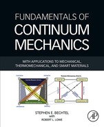
Consider an arbitrary part S![]() of body B
of body B![]() that occupies a region P
that occupies a region P![]() in the present configuration at time t. Let P
in the present configuration at time t. Let P![]() be divided into two regions, P1
be divided into two regions, P1![]() and P2
and P2![]() , separated by a surface σ (see Figure 4.1). Define ∂P′
, separated by a surface σ (see Figure 4.1). Define ∂P′![]() and ∂P′′
and ∂P′′![]() so that ∂P=∂P′∪∂P′′
so that ∂P=∂P′∪∂P′′![]() . Then, P=P1∪P2
. Then, P=P1∪P2![]() , ∂P=∂P′∪∂P′′
, ∂P=∂P′∪∂P′′![]() , ∂P1=∂P′∪σ
, ∂P1=∂P′∪σ![]() , ∂P2=∂P′′∪σ
, ∂P2=∂P′′∪σ![]() .
.
 into two regions, P1
 and P2
 , separated by a surface σ.
Applying balance of linear momentum to the three regions P![]() , P1
, P1![]() , and P2
, and P2![]() , we obtain
, we obtain
ddt∫P˙xρdv=∫Pbρdv+∫∂Pt(n)da,
ddt∫P1˙xρdv=∫P1bρdv+∫∂P′∪σt(n)da,

ddt∫P2˙xρdv=∫P2bρdv+∫∂P″∪σt(n)da.

Adding (b) and (c) then subtracting (a) gives
∫σ[t(n)+t(−n)]da=0.

In (d) we have noted that the outward normal of σ, when considered as a part of the boundary of P1![]() , is directly opposed to the outward normal of σ when considered as a part of the boundary of P2
, is directly opposed to the outward normal of σ when considered as a part of the boundary of P2![]() . Assuming the traction is a continuous function of x and n, so that we can use the two-dimensional localization theorem, (d) implies
. Assuming the traction is a continuous function of x and n, so that we can use the two-dimensional localization theorem, (d) implies
t(n)=−t(−n).
(Traction vectors on opposite sides of the same surface are equal in magnitude, and opposite in direction.)
Consider now a family of similar tetrahedra T![]() with heights hp and a common vertex at some point ox (see Figure 4.2). Sides i are perpendicular to the xi directions and have outward normals −ei. The remaining side has outward normal on. From geometry, areas S
with heights hp and a common vertex at some point ox (see Figure 4.2). Sides i are perpendicular to the xi directions and have outward normals −ei. The remaining side has outward normal on. From geometry, areas S![]() , S1
, S1![]() , S2
, S2![]() , and S3
, and S3![]() are related by
are related by
Si=S(on·ei)=Sni.
The volumes of the tetrahedra are
V=13hpS.
It is assumed that each of the tetrahedra lies completely within the region R![]() occupied by B
occupied by B![]() in the present configuration. By virtue of the transport theorem (4.20) and the local form of conservation of mass (presented later in Section 4.8), (a) becomes
in the present configuration. By virtue of the transport theorem (4.20) and the local form of conservation of mass (presented later in Section 4.8), (a) becomes
∫P¨xρdv=∫Pbρdv+∫∂Pt(n)da.
Applying (h) to a tetrahedron T![]() gives
gives
∫T(x¨−b)ρdv=∫ΣSit(−ei)da+∫St(on)da.
∫T(x¨−b)ρdv=∫St(on)da−∫ΣSit(ei)da.
Recall that the specific body force b and density ρ are assumed bounded throughout R![]() . The acceleration ¨x
. The acceleration ¨x![]() is also assumed bounded. Then,
is also assumed bounded. Then,
|∫T(¨x−b)ρdv|≤∫T|¨x−b|ρdv(by a theorem of analysis)=∫TKdv(by boundedness)=K∫Tdv=KShp3(using(g)),

where K is some number. Assuming that t is a continuous function of x and t, the mean value theorem and (f) imply that
∫St(on)da−∫ΣSit(ei)da=t*(on)S−t*(ei)Si=[t*(on)−t*(ei)ni]S,

where t*(on) and t*(ei) stand for some specific interior values of the traction vectors on the faces S![]() and Si
and Si![]() , respectively. From (j) to (l),
, respectively. From (j) to (l),
13KShp≥|∫T|¨x−b|ρdv|=|∫St(on)da−∫ΣSit(ei)da|=|t*(on)−t*(ei)ni|S,

so
|t*(on)−t*(ei)ni|≤13Khp.
As we consider smaller and smaller tetrahedra, hp → 0, and
limhp→0|t*(on)−t*(ei)ni|=0,
where t*(on) and t*(ei) are evaluated at the point ox, which is the common vertex of the family of tetrahedra. From (m), we see that in the limit hp → 0, t*(on) − t*(ei)ni must be the zero vector, i.e.,
t*(on)=t*(ei)oni,
where t*(ei)o denotes the value of t*(ei) at the point ox. Since (n) must hold at any point ox and corresponding to any direction on, without ambiguity, we may delete the star, replace ox and on by x and n, and write
t(n)=t(ei)ni.
We define Tki by
Tki=t(ei)·ek,
and denote the components of t(n) by
tk=t·ek.
Taking the inner product of (o) with the unit vector ek thus gives
tk=t(ei)ni·ek=Tkini.
Equation (p) is the Cartesian component form of
t=Tnort(x,t,n)=T(x,t)n.

 , S2
, S2 , and S3
 have outward unit normals −e1, −e2, and −e3, respectively, while side S has outward unit normal on.
Recall from Section 4.4 that the heat flux h out of the surface ∂P![]() is, in general, a function of position x, time t, and the geometry of the surface, i.e.,
is, in general, a function of position x, time t, and the geometry of the surface, i.e.,
h=˜h(x,t,geometry of surface).
We restrict our attention to a particular type of heat flow through the boundary ∂P![]() , namely, one such that the heat flux h is the same for all like-oriented surfaces with a common tangent plane at x and t, so (4.29) becomes
, namely, one such that the heat flux h is the same for all like-oriented surfaces with a common tangent plane at x and t, so (4.29) becomes
h=˜h(x,t,n).
We further assume that h is a continuous function of x, t, and n. Then, as a consequence of the conservation laws of mass (4.11a), linear momentum (4.11b), and energy (4.19), and our boundedness assumptions, it can be shown (refer to Problem 4.4) that the dependence of h on n in (4.30) must be linear, i.e.,
˜h(x,t,n)=˜q(x,t)·norh=q·n.
The vector q in (4.31) is called the heat flux vector.
Problem 4.4
Show that h = q · n.
Consider once again the regions P![]() , P1
, P1![]() , and P2
, and P2![]() shown in Figure 4.1. Applying the first law of thermodynamics to these three regions, we have
shown in Figure 4.1. Applying the first law of thermodynamics to these three regions, we have
ddt∫P(˙x·˙x2+ε)ρdv=∫P(b·v+r)ρdv+∫∂P[t(n)·v−h(n)]da,
ddt∫P1(˙x·˙x2+ε)ρdv=∫P1(b·v+r)ρdv+∫∂P′∪σ[t(n)·v−h(n)]da,
ddt∫P2(˙x·˙x2+ε)ρdv=∫P2(b·v+r)ρdv+∫∂P″∪σ[t(n)·v−h(n)]da,

Adding (b) and (c) then subtracting (a) gives
∫σ[t(n)+t(−n)]·vda+∫σ[h(n)+h(−n)]da=0.

In (d) we have noted that the outward normal of σ when considered as a part of ∂P1![]() is directly opposed to the outward normal of σ when considered as a part of ∂P2
is directly opposed to the outward normal of σ when considered as a part of ∂P2![]() . The result
. The result
t(n)=−t(−n)
from Problem 4.3 implies that (d) becomes
∫σ[h(n)+h(−n)]da=0.

Assuming continuity of h, it then follows that
h(n)=−h(−n).
(The heat leaving one part equals the heat entering the other part.)
By virtue of the transport theorem (4.20) and the local form of conservation of mass (presented later in Section 4.8), (a) reduces to
∫P(v·˙v+˙ε)ρdv=∫P(b·v+r)ρdv+∫∂P[t(n)·v−h(n)]da.

Applying this to the tetrahedron T![]() in Figure 4.2 gives
in Figure 4.2 gives
∫T(v·˙v+˙ε−b·v−r)ρdv=∫ΣSi[t(−ei)·v−h(−ei)]da+∫S[t(on)·v−h(on)]da,

or, using (e),
∫T(v·˙v+˙ε−b·v−r)ρdv=∫ΣSi[−t(ei)·v+h(ei)]da+∫S[t(on)·v−h(on)]da.

We assume that ε, ˙ε![]() , v, ˙v
, v, ˙v![]() , and r are bounded, so
, and r are bounded, so
|∫T(v·˙v+˙ε−b·v−r)ρdv|≤MShp3
for some number M. Therefore, from (f), (g), and the mean value theorem, we have
13MShp≥|∫ΣSi[−t(ei)·v+h(ei)]da+∫S[t(on)·v−h(on)]da|=|[t*(on)·v*−h*(on)]S+[−t*(ei)·v*(i)+h*(ei)]Si|=|t*(on)·v*−t*(ei)ni·v*(i)−h*(on)+h*(ei)ni|S,

where t*(on), v*, and h*(on) stand for some specific interior values on face S![]() , and t*(ei), v*(i), and h*(ei) stand for some specific values on faces Si
, and t*(ei), v*(i), and h*(ei) stand for some specific values on faces Si![]() . Then
. Then
limhp→0|t*(on)·v*−t*(ei)ni·v*(i)−h*(on)+h*(ei)ni|=0,
so in the limit,
t*(on)·v*−t*(ei)ni·v*(i)−h*(on)+h*(ei)ni=0.
In the limit, v* = v*(i) = v(ox, t), and so (h) becomes
[t*(on)−t*(ei)ni]·v*−h*(on)+h*(ei)ni=0.
Recall from Problem 4.3 that
t*(on)=t*(ei)oni.
As a consequence, (i) becomes
h*(on)=h*(ei)niorh(n)+h(ei)ni.
We define qi by
qi=h(ei)
so that (j) is written as
h(n)=qini.
Equation (k) is the Cartesian component form of
h=q·norh(x,t,n)=q(x,t)·n.
4.7 The energy theorem and stress power
Recall from Section 4.3 the Eulerian representations of the mechanical integral conservation laws:
ddt∫Pρdv=0,

ddt∫Pvρdv=∫Pbρdv+∫∂PTnda,

ddt∫Px×vρdv=∫Px×bρdv+∫∂Px×Tda,

where we have used t = Tn (result (4.26)). As a consequence of these mechanical conservation laws, it can be shown (refer to Problem 4.7) that the rate of work of all external forces acting on P![]() and its boundary ∂P
and its boundary ∂P![]() minus the rate of increase of the kinetic energy is equal to the total stress power of P
minus the rate of increase of the kinetic energy is equal to the total stress power of P![]() :
:
∫Pb·vρdv+∫∂Pt·vda−ddt∫P12v·vρdv+∫PT·Ddv.
This result, called the energy theorem, is a mechanical result: it follows only from the mechanical laws (4.32a)–(4.32c) and does not depend on conservation of energy. The scalar quantity T · D in (4.33) is called the stress power P, i.e.,
P=T·D.
Problem 4.7
Verify that the Eulerian (or spatial) form of the energy theorem
∫Pb·vρdv+∫∂Pt·vda−ddt∫P12v·vρdv=∫PT·Ddv

is a consequence of the mechanical conservation laws of mass, linear momentum, and angular momentum.
To begin, we consider the second term on the left-hand side of the energy theorem:
∫∂Pt·vda=∫∂PTn·vda(result(4.26))=∫∂PTTv·nda(definition(2.13))=∫Pdiv(TTv)dv(divergence theorem(2.104)2)=∫P(T·gradv+v·divT)dv(result(2.99)4).

Note that this result is consistent with (2.105). Also note that grad and div are the gradient and divergence calculated with respect to the present configuration. Next, considering the third term on the left-hand side of the energy theorem, we have
ddt∫P12v·vρdv=∫P(12.¯v·vρ+12v·vρdivv)dv(transport theorem(4.20))=∫P[ρ˙v·v+12v·v(˙ρ+ρdivv)]dv(product rule(3.22))=∫Pρ˙v·vdv(conservation of mass(4.36a)).

After assembling these results, the left-hand side of the energy theorem becomes
∫P[(ρb+divT−ρ˙v)·v+T·gradv]dv.
By virtue of the local form of conservation of linear momentum (4.36b), this further reduces to
∫PT·gradvdv.

Then,
∫PT·gradvdv=∫PT·Ldv(definition(3.56))=∫PT·(D+W)dv(decomposition(3.57))=∫P(T·D+T·W)dv(property(2.6)3)=∫PT·Ddv(result(2.44)),

where, in the last step, we have exploited the local form of conservation of angular momentum (4.36c), which demands that T is symmetric; recall that W is skew by construction. (Note that we were able to employ the distributive property (2.6)3 of the inner product in the next-to-last step since we demonstrated in Problem 2.35 that the set of all second-order tensors is an inner product space.) Thus, we conclude that
∫Pb·vρdv+∫∂Pt·vda−ddt∫P12v·vρdv=∫PT·Ddv.
