
Modeling of Thermo-Electro-Magneto-Mechanical Behavior, with Application to Smart Materials
Sushma Santapuri; Robert L. Lowe; Stephen E. Bechtel Department of Mechanical and Aerospace Engineering, The Ohio State University Columbus, OH
Abstract
A key feature of smart materials is their ability to convert energy from one form into another. For instance, piezoelectric materials deform when exposed to an electric field, thus converting electrical energy to mechanical energy. Other common smart materials include magnetostrictives, magnetorheological fluids, shape memory alloys, and electroactive polymers. These materials couple different physical effects, e.g., thermal, electrical, magnetic, and/or mechanical. In this chapter, we present a continuum framework that lays the groundwork for modeling a broad range of smart materials exhibiting coupled thermal, electrical, magnetic, and/or mechanical behavior. This framework has the breadth to accommodate large deformations (i.e., geometric nonlinearities), anisotropy, and nonlinear constitutive response (i.e., material nonlinearity). We devote special attention to developing the fundamental laws of continuum electrodynamics and presenting key aspects of thermodynamic constitutive modeling. For instance, we show how the thermodynamic formalism that produced constitutive models for classical elastic solids and viscous fluids can also be used to facilitate the constitutive modeling of smart materials with coupled thermo-electro-magneto-mechanical (TEMM) behavior. Finally, we illustrate that our modeling approach provides an overarching framework that encompasses many well-known types of smart material behavior. For instance, we explicitly demonstrate that the linear theory of piezoelectricity falls out as a special case of our more general finite-deformation TEMM framework, much the same way linear elasticity falls out of finite-deformation elasticity.
In this chapter, we present a continuum approach to modeling smart materials. A key feature of smart materials is their ability to convert energy from one form into another. For instance, piezoelectric materials deform when exposed to an electric field, thus converting electrical energy to mechanical energy. Other common smart materials include magnetostrictives, magnetorheological fluids, shape memory alloys, and electroactive polymers. These materials couple different physical effects, e.g., thermal, electrical, magnetic, and/or mechanical. Owing to their unique properties, smart materials are implemented in a wide variety of automotive, aerospace, and biomedical applications, to name but a few.
Compared with classical elastic solids and viscous fluids (refer to Chapters 4–8), additional balance laws (e.g., Maxwell's equations) are required to model the complex multiphysics behavior of smart materials. Also, the thermomechanical balance laws (i.e., linear momentum, angular momentum, and energy) must be modified to account for contributions from electromagnetic fields. Finally, the constitutive equations that describe the response of smart materials should highlight the coupling of different physical effects. For example, stress in a piezoelectric material is a function of both strain and electric field.
In what follows, we present a unified continuum framework that lays the groundwork for modeling a broad range of smart materials exhibiting coupled thermal, electrical, magnetic, and/or mechanical behavior. This framework has the breadth to accommodate dynamic electromagnetic fields, large deformations (i.e., geometric nonlinearities), anisotropy, and nonlinear constitutive response (i.e., material nonlinearity). We devote special attention to developing the fundamental laws of continuum electrodynamics and presenting key aspects of thermodynamic constitutive modeling. For instance, we show how the thermodynamic formalism that produced constitutive models for classical elastic solids (refer to Chapter 6) and viscous fluids (refer to Chapter 7) can also be used to facilitate the constitutive modeling of smart materials with thermo-electro-magneto-mechanical (TEMM) behavior. Finally, we illustrate that our modeling approach provides an overarching framework that encompasses many well-known types of smart material behavior. For instance, we explicitly demonstrate that the linear theory of piezoelectricity falls out as a special case of our more general finite-deformation TEMM framework, in much the same way linear elasticity falls out of finite-deformation elasticity.
Although some of the concepts presented in this chapter are introduced in earlier parts of the book, they are restated here so that this chapter is essentially self-contained.
9.1 The fundamental laws of continuum electrodynamics: integral forms
In this section, we present the fundamental laws of continuum electrodynamics, i.e., the first principles for a deformable, polarizable, magnetizable, conductive thermo-electro-magneto-mechanical (TEMM) material. As was done in Chapter 4, the first principles are postulated at four different levels: primitive, material, integral, and pointwise. In particular, we begin by explicitly stating the first principles in their most primitive or fundamental form. These primitive statements are then expressed mathematically in material form. The material form is global, i.e., valid on the body as a whole and all subsets.1 Specializing to a continuum leads to a corresponding set of integral equations. Boundedness and continuity then allow these integral equations to be localized, i.e., expressed in a pointwise fashion. Note that we carefully progress from primitive statements to pointwise equations, rather than starting directly with a set of pointwise equations, since (1) the pointwise equations must be derivable from an integral set and (2) the assumptions for continuum models are customarily imposed on the integral form [30, 31].
9.1.1 Notation and nomenclature
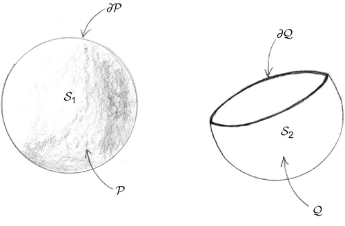
We now present the notation necessary to describe the geometry of the deformable TEMM body. We label the body B![]() and two arbitrary subsets S1
and two arbitrary subsets S1![]() and S2
and S2![]() .2 Subset S1
.2 Subset S1![]() is bounded by a closed material surface, while subset S2
is bounded by a closed material surface, while subset S2![]() is bounded by a closed material curve; see Figure 9.1. As will soon be evident, both closed material surfaces and closed material curves are required to formulate integral statements of the fundamental laws of continuum electrodynamics.
is bounded by a closed material curve; see Figure 9.1. As will soon be evident, both closed material surfaces and closed material curves are required to formulate integral statements of the fundamental laws of continuum electrodynamics.
 and S2
 as seen in the present configuration. Subset S1
 is an open material volume P
 bounded by a closed material surface ∂P
 , while subset S2
 is an open material surface Q
 bounded by a closed material curve ∂Q
 .
.In the reference configuration, body B![]() occupies open volume RR
occupies open volume RR![]() of e ∂RR
of e ∂RR![]() . Subset S1
. Subset S1![]() occupies open volume PR⊂RR
occupies open volume PR⊂RR![]() , bounded by closed surface ∂PR
, bounded by closed surface ∂PR![]() , and subset S2
, and subset S2![]() occupies open surface QR⊂RR
occupies open surface QR⊂RR![]() , bounded by closed curve ∂QR
, bounded by closed curve ∂QR![]() .
.
In the present configuration at time t, body B![]() occupies open material volume R
occupies open material volume R![]() , bounded by closed material surface ∂R
, bounded by closed material surface ∂R![]() . Subset S1
. Subset S1![]() occupies open material volume P⊂R
occupies open material volume P⊂R![]() , bounded by closed material surface ∂P
, bounded by closed material surface ∂P![]() , and subset S2
, and subset S2![]() occupies open material surface Q⊂R
occupies open material surface Q⊂R![]() , bounded by closed material curve ∂Q
, bounded by closed material curve ∂Q![]() .3
.3
9.1.2 Conservation of mass
Primitively, conservation of mass postulates that the mass M![]() of every subset of the body B
of every subset of the body B![]() is constant throughout its motion, or, equivalently, the time rate of change of the mass of every subset is zero. Applying this primitive statement to arbitrary subset S1
is constant throughout its motion, or, equivalently, the time rate of change of the mass of every subset is zero. Applying this primitive statement to arbitrary subset S1![]() allows us to express conservation of mass mathematically in material form:
allows us to express conservation of mass mathematically in material form:
ddtM(S1,t)=0orM(S1)≡independent oft.
Specializing to a continuum, the approach taken heretofore in this book, allows us to express the mass M![]() of subset S1
of subset S1![]() in Eulerian and Lagrangian integral forms, i.e.,
in Eulerian and Lagrangian integral forms, i.e.,
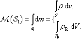
M(S1)=∫S1dm={∫Pρdv,∫PRρRdV.
Thus, specializing to a continuum is tantamount to a smoothness assumption on the mass M![]() ; refer to Section 4.2. The Eulerian integral representation (top of (9.2)) corresponds to subset S1
; refer to Section 4.2. The Eulerian integral representation (top of (9.2)) corresponds to subset S1![]() as seen in its present configuration, while the Lagrangian integral representation (bottom of (9.2)) corresponds to S1
as seen in its present configuration, while the Lagrangian integral representation (bottom of (9.2)) corresponds to S1![]() as seen in its reference configuration.4 In (9.2), dv and dV are volume elements in the present and reference configurations (refer to Section 3.6), and ρ and ρR are the mass densities in the present and reference configurations (refer to Section 4.1). Note that ρ has units of mass per present volume, while ρR has units of mass per reference volume (see Table 9.1). Both ρ and ρR are bounded, continuous functions of space and time.
as seen in its reference configuration.4 In (9.2), dv and dV are volume elements in the present and reference configurations (refer to Section 3.6), and ρ and ρR are the mass densities in the present and reference configurations (refer to Section 4.1). Note that ρ has units of mass per present volume, while ρR has units of mass per reference volume (see Table 9.1). Both ρ and ρR are bounded, continuous functions of space and time.
Table 9.1
Units for Thermal, Electrical, Magnetic, and Mechanical Quantities
| Type | Quantity | Representation | Symbol | Fundamental Units | Derived Units | SI Units |
| Electrical | Vacuum permittivity | εo | C2T2ML3P |
CapacitancePresent length |
FaradMeter | |
| Electric field | Referential | eR | ML2PLRT2C |
ForceCharge·Present lengthReference length |
NewtonCoulomb≡VoltMeter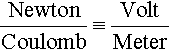 | |
| Spatial | e* | MLPCT2 |
ForceCharge |
NewtonCoulomb≡VoltMeter | ||
| Electric polarization | Referential | pR | CL2R |
ChargeReference area |
CoulombMeter2 | |
| Spatial | p* | CL2P |
ChargePresent area |
CoulombMeter2 | ||
| Electric displacement | Referential | dR | CL2R |
ChargeReference area |
CoulombMeter2 | |
| Spatial | d* | CL2P |
ChargePresent area |
CoulombMeter2 | ||
| Free charge density | Referential | σR | CL3R |
ChargeReference volume |
CoulombMeter3 | |
| Spatial | σ* | CL3P |
ChargePresent volume |
CoulombMeter3 | ||
| Conductive current density | Referential | jR | CL2RT |
CurrentReference area |
AmpereMeter2 | |
| Spatial | j* | CL2PT |
CurrentPresent area |
AmpereMeter2 | ||
| Magnetic | Vacuum permeability | μo | MLPC2 |
InductancePresent length |
HenryMeter | |
| Magnetic field | Referential | hR | CLRT |
CurrentReference length |
AmpereMeter | |
| Spatial | h* | CLPT |
CurrentPresent length |
AmpereMeter | ||
| Magnetization | Referential | mR | CLRT |
CurrentReference length |
AmpereMeter | |
| Spatial | m* | CLPT |
CurrentPresent length |
AmpereMeter | ||
| Magnetic flux density | Referential | bR | ML2PL2RTC |
Magnetic fluxReference area |
WeberMeter2≡Tesla | |
| Spatial | b* | MTC |
Magnetic fluxPresent area |
WeberMeter2≡Tesla | ||
| Mechanical | Mass density | Referential | ρR | ML3R |
MassReference volume |
KilogramMeter3 |
| Spatial | ρ | ML3P |
MassPresent volume |
KilogramMeter3 | ||
| Traction | Referential | tR | MLPL2RT2 |
ForceReference area |
NewtonMeter2≡Pascal | |
| Spatial | t | MLPT2 |
ForcePresent area |
NewtonMeter2≡Pascal | ||
| Stress | Referential | P | MLPL2RT2 |
ForceReference area |
NewtonMeter2≡Pascal | |
| Spatial | T | MLPT2 |
ForcePresent area |
NewtonMeter2≡Pascal | ||
| Velocity | v | LPT |
MeterSecond | |||
| Deformation gradient | F | LPLR |
||||
| Green's deformation | C | L2PL2R |
||||
| Volumetric deformation | J | L3PL3R |
||||
| Thermal | Heat flux rate | Referential | hR | ML2PL2RT3 |
EnergyReference area·time |
WattMeter2 |
| Spatial | h | MT3 |
EnergyPresent area·time |
WattMeter2 | ||
| Heat flux vector | Referential | qR | ML2PL2RT3 |
EnergyReference area·time |
WattMeter2 | |
| Spatial | q | MT3 |
EnergyPresent area·time |
WattMeter2 | ||
| Temperature | Θ | θ | Kelvin | |||
| Specific internal energy | ε | L2PT2 |
EnergyMass |
JouleKilogram | ||
| Specific entropy | η | L2PT2θ |
EnergyMass·temperature |
JouleKilogram·kelvin |


Note that M is mass, LPis present length, LRis reference length, T is time, θ is temperature, and C is charge.
To perform the integrations in (9.2), it is natural to consider ρ in its Eulerian description, i.e., as a function of x and t, and to consider ρR in its Lagrangian description, i.e., as a function of X and t, although both ρ and ρR can be expressed using either an Eulerian or a Lagrangian description. Recall that X and x are the reference and present positions of a continuum particle, related through the motion x = χ(X, t) (refer to Section 3.1).
Use of (9.2) in (9.1) leads to Eulerian and Lagrangian integral representations of conservation of mass:
ddt∫Pρdv=0,
∫Pρdv=∫PRρRdV.

These integral statements are valid for any open volume P![]() in the present configuration and corresponding open volume PR
in the present configuration and corresponding open volume PR![]() in the reference configuration. Note that (9.3a) and (9.3b) are identical to their counterparts in the thermomechanical theory (refer to Chapter 4).
in the reference configuration. Note that (9.3a) and (9.3b) are identical to their counterparts in the thermomechanical theory (refer to Chapter 4).
9.1.3 Balance of linear momentum
Balance of linear momentum postulates that the time rate of change of the linear momentum L![]() of any subset of the body is equal to the resultant external force f acting on that subset. Applying this primitive statement to subset S1
of any subset of the body is equal to the resultant external force f acting on that subset. Applying this primitive statement to subset S1![]() gives the material form:
gives the material form:
ddtL(S1,t)=f(S1,t).
Assuming smoothness of L![]() , we write its Eulerian and Lagrangian integral representations:
, we write its Eulerian and Lagrangian integral representations:
L(S1,t)={∫Pvρdv,∫PRvρRdV,

where v is the velocity of a continuum particle at the present time t, and the integrands are continuous, bounded functions of space and time. As was done in Section 4.2, it is assumed that the resultant external force f can be additively decomposed into a body force and a contact force. The effects of electromagnetism are modeled through an electromagnetic contribution to the body force [32, 33] so that
f(S1,t)={∫P(fm+fem)ρdv+∫∂Ptda,∫PR(fm+fem)ρRdV+∫∂PRtRdA,

where fm is the mechanically induced body force per unit mass, fem is the electro-magnetically induced body force per unit mass, t and tR are the spatial and referential tractions (refer to Section 4.9), and da and dA are area elements in the present and reference configurations (refer to Section 3.6).5 Elaborating, t is the traction acting on surface ∂P![]() in the present configuration measured per unit area of ∂P
in the present configuration measured per unit area of ∂P![]() , whereas tR is the traction acting on surface ∂P
, whereas tR is the traction acting on surface ∂P![]() in the present configuration but measured per unit area of the corresponding surface ∂PR
in the present configuration but measured per unit area of the corresponding surface ∂PR![]() in the reference configuration. Thus, t has units of force per present area, while tR has units of force per reference area (see Table 9.1).
in the reference configuration. Thus, t has units of force per present area, while tR has units of force per reference area (see Table 9.1).
Use of (9.5) and (9.6) in (9.4) gives Eulerian and Lagrangian integral representations of balance of linear momentum:
ddt∫Pvρdv=∫P(fm+fem)ρdv+∫∂Ptda,
ddt∫PRvρRdV=∫PR(fm+fem)ρRdV+∫∂PRtRdA.

Comparing (9.7a) and (9.7b) with their counterparts in the thermomechanical theory (refer to Chapter 4), we see that (9.7a) and (9.7b) contain an additional body force fem.
9.1.4 Balance of angular momentum
Balance of angular momentum postulates that the time rate of change of the angular momentum H0 of any subset of the body about the origin 0 is equal to the resultant external moment M0 acting on that subset about the origin 0. In material form:
ddtH0(S1,t,0)=M0(S1,t,0).

Assuming that H0 is smooth leads to Eulerian and Lagrangian integral representations of the angular momentum about 0, i.e.,
H0(S1,t,0)={∫Px×vρdv,∫PRx×vρRdV.

The integrands in (9.9) are continuous, bounded functions of space and time. Similarly, smoothness of M0 implies that
M0(S1,t,0)={∫Px×(fm+fem)ρdv+∫∂Px×tda+∫Pcemρdv,∫PRx×(fm+fem)ρRdV+∫∂PRx×tRdA+∫PRcemρRdV.

Following [32, 33], an electromagnetically induced body couple per unit mass cem is included in (9.10) to model the effects of electromagnetism. Note that the first two terms in (9.10)1 and (9.10)2 represent the moment about 0 due to the resultant external force f, the first term being a contribution from the body force and the second term being a contribution from the contact force.
Use of (9.9) and (9.10) in (9.8) gives Eulerian and Lagrangian integral representations of balance of angular momentum:
ddt∫Px×vρdv=∫Px×(fm+fem)ρdv+∫∂Px×tda+∫Pcemρdv,

ddt∫PRx×vρRdV=∫PRx×(fm+fem)ρRdV+∫∂PRx×tRdA+∫PRcemρRdV.

Comparing (9.11a) and (9.11b) with their counterparts in the thermomechanical theory (refer to Chapter 4), we see that (9.11a) and (9.11b) contain additional moments due to (1) the electromagnetic body force fem and (2) the electromagnetic body couple cem.
9.1.5 First law of thermodynamics
The first law of thermodynamics (or conservation of energy) postulates that the time rate of change of the total energy (i.e., kinetic energy K plus internal energy E) of any subset of the body is equal to the rate of work R generated by the resultant external force acting on that subset plus the rate of all other energies A![]() (e.g., heat, electromagnetic, chemical) entering or exiting that subset. In material form,
(e.g., heat, electromagnetic, chemical) entering or exiting that subset. In material form,
ddt(K(S1,t)+E(S1,t))=R(S1,t)+A(S1,t).
Assuming that the kinetic and internal energies of part S1![]() are smooth implies that
are smooth implies that
K(S1,t)={∫P12v·vρdv,∫PR12v·vρRdV,E(S1,t)={∫Pερdv,∫PRερRdV,

where ε is the specific internal energy (or internal energy per unit mass), and the integrands are bounded, continuous functions of space and time. The rate of work R generated by the resultant external force f can be additively decomposed into contributions from the body force and the contact force, i.e.,
R(S1,t)={∫P(fm+fem)·vρdv+∫∂Pt·vda,∫PR(fm+fem)·vρRdV+∫∂PRtR·vdA.

Following [32, 33], the auxiliary energy rate A![]() is additively decomposed into three contributions, two from radiation and one from conduction: the rate of heat absorption throughout the volume, the rate of electromagnetic energy absorption throughout the volume, and the rate of heat entering through the boundary, i.e.,
is additively decomposed into three contributions, two from radiation and one from conduction: the rate of heat absorption throughout the volume, the rate of electromagnetic energy absorption throughout the volume, and the rate of heat entering through the boundary, i.e.,
A(S1,t)={∫Prtρdv+∫Premρdv−∫∂Phda,∫PRrtρRdV+∫PRremρRdV−∫∂PRhRdA,

where rt is the specific heat supply rate, rem is the specific electromagnetic energy supply rate, and hR and h are the referential and spatial heat flux rates (refer to Section 4.9.3).6 Elaborating, h is the rate of heat flow out of the present boundary ∂P![]() measured per unit area of the present boundary ∂P
measured per unit area of the present boundary ∂P![]() . Conversely, hR is the rate of heat flow out of the present boundary ∂P
. Conversely, hR is the rate of heat flow out of the present boundary ∂P![]() , but measured per unit area of the corresponding boundary ∂PR
, but measured per unit area of the corresponding boundary ∂PR![]() in the reference configuration. Thus, h has units of energy per time per present area, while hR has units of energy per time per reference area (see Table 9.1).
in the reference configuration. Thus, h has units of energy per time per present area, while hR has units of energy per time per reference area (see Table 9.1).
Use of (9.13)–(9.15) in (9.12) yields Eulerian and Lagrangian integral representations of the first law of thermodynamics:
ddt∫P12v·vρdv+ddt∫Pερdv=∫P(fm+fem)·vρdv+∫∂Pt·vda+∫P(rt+rem)ρdv−∫∂Phda,
ddt∫PR12v·vρRdV+ddt∫PRερRdV=∫PR(fm+fem)·vρRdV+∫∂PRtR·vdA+∫PR(rt+rem)ρRdV−∫∂PRhRdA.

Comparing (9.16a) and (9.16b) with their counterparts in the thermomechanical theory (refer to Chapter 4), we see that (9.16a) and (9.16b) contain additional energy contributions from (1) the work due to the electromagnetic body force fem and (2) the electromagnetic energy supply rem.
9.1.6 Second law of thermodynamics
In this chapter—as was done in the thermomechanical theory of Chapter 4—we adopt the Clausius-Duhem inequality as our particular statement of the second law of thermodynamics. The Clausius-Duhem inequality postulates that the rate of change of the entropy N![]() of any subset of the body is greater than or equal to the rate of entropy generation R
of any subset of the body is greater than or equal to the rate of entropy generation R![]() due to the radiative heat supply minus the rate of entropy loss H
due to the radiative heat supply minus the rate of entropy loss H![]() due to the outward heat flux. Applying this primitive statement of the second law to subset S1
due to the outward heat flux. Applying this primitive statement of the second law to subset S1![]() yields the material form:
yields the material form:
ddtN(S1,t)≥R(S1,t)−H(S1,t).
Specializing to a continuum and assuming smoothness of N(S1,t)![]() , R(S1,t)
, R(S1,t)![]() , and H(S1,t)
, and H(S1,t)![]() , we can write
, we can write
N(S1,t)={∫Pηρdv,∫PRηρRdV,R(S1,t)={∫PrtΘρdv,∫PRrtΘρRdV,

and
H(S1,t)={∫∂PhΘda,∫∂PRhRΘdA,

where η is the specific entropy (or entropy per unit mass) and Θ is the absolute temperature. The Eulerian integral representations of N(S1,t)![]() , R(S1,t)
, R(S1,t)![]() , and H(S1,t)
, and H(S1,t)![]() (top of (9.18) and (9.19)) correspond to subset S1
(top of (9.18) and (9.19)) correspond to subset S1![]() as seen in its present configuration, while the Lagrangian integral representations of these quantities (bottom of (9.18) and (9.19)) correspond to subset S1
as seen in its present configuration, while the Lagrangian integral representations of these quantities (bottom of (9.18) and (9.19)) correspond to subset S1![]() as seen in its reference configuration.
as seen in its reference configuration.
Use of (9.18) and (9.19) in (9.17) leads to Eulerian and Lagrangian integral representations of the Clausius-Duhem inequality:
ddt∫Pηρdv≥∫PrtΘρdv−∫∂PhΘda,
ddt∫PRηρRdV≥∫PRrtΘρRdV−∫∂PRhRΘdA.

Note that these integral statements are valid for any open volume P![]() bounded by closed surface ∂P
bounded by closed surface ∂P![]() in the present configuration, or corresponding open volume PR
in the present configuration, or corresponding open volume PR![]() bounded by closed surface ∂PR
bounded by closed surface ∂PR![]() in the reference configuration. Also note that (9.20a) and (9.20b) are identical to their counterparts in the thermomechanical theory (refer to Chapter 4).
in the reference configuration. Also note that (9.20a) and (9.20b) are identical to their counterparts in the thermomechanical theory (refer to Chapter 4).
9.1.7 Conservation of electric charge
Conservation of charge postulates that the time rate of change of the total electric charge (i.e., free charge Σ plus bound charge Σb) within any closed material surface is equal to the sum of the free (or conductive) current J![]() and the polarization current Jp
and the polarization current Jp![]() entering that surface. Applying this primitive statement of the law to subset S1
entering that surface. Applying this primitive statement of the law to subset S1![]() (an open material volume bounded by a closed material surface) allows us to express conservation of charge mathematically in material form:
(an open material volume bounded by a closed material surface) allows us to express conservation of charge mathematically in material form:
ddt(Σ(S1,t)+Σb(S1,t))=J(S1,t)+Jp(S1,t).
Loosely, free charges are unpaired and “free” to move; this motion gives rise to the conductive current. Conversely, bound charges are paired, and are thus “bound” to a particular atom. When a material experiences a spatially varying polarization, the bound charges realign; if this polarization is also time varying, a polarization current arises.
Physically, the conductive current J(S1,t)![]() always enters and exits subset S1
always enters and exits subset S1![]() at time t through its present surface ∂P
at time t through its present surface ∂P![]() , but we are free to label this surface by its reference location ∂PR
, but we are free to label this surface by its reference location ∂PR![]() instead. Similarly, the free charge ∑(S1,t)
instead. Similarly, the free charge ∑(S1,t)![]() always resides in present volume P
always resides in present volume P![]() , but we are free to label this volume by its reference location PR
, but we are free to label this volume by its reference location PR![]() instead. Exploiting this freedom in how the geometry of S1
instead. Exploiting this freedom in how the geometry of S1![]() is labeled allows us to write Eulerian and Lagrangian integral representations of the free charge, bound charge, conductive current, and polarization current, i.e.,
is labeled allows us to write Eulerian and Lagrangian integral representations of the free charge, bound charge, conductive current, and polarization current, i.e.,
Σ(S1,t)={∫Pσ*dv,∫PRσRdV,Σb(S1,t)={−∫Pdivp*dv,−∫PRDivpRdV,

J(S1,t)={−∫∂Pj*·nda,−∫∂PRjR·NdA,Jp(S1,t)={−ddt∫∂Pp*·nda,−ddt∫∂PRpR·NdA,

where n and N are outward unit normals in the present and reference configurations (refer to Section 3.6), “div” denotes the Eulerian divergence (i.e., the divergence calculated with respect to the present configuration), and “Div” denotes the Lagrangian divergence (i.e., the divergence calculated with respect to the reference configuration). Note that the minus signs in (9.23) are required to maintain consistency in our sign convention: positive J![]() denotes current flowing into the boundary (see (9.21)), whereas positive j* · n implies that current is flowing out of the boundary (n is an outward unit normal).
denotes current flowing into the boundary (see (9.21)), whereas positive j* · n implies that current is flowing out of the boundary (n is an outward unit normal).
In (9.22) and (9.23), σ* and σR are denoted the spatial free charge density and referential free charge density, j* and jR the spatial conductive current density and referential conductive current density, and p* and pR the spatial electric polarization and referential electric polarization. All are bounded, continuous functions of space and time. Recall that the spatial and referential representations of a particular quantity are different since they are associated with different labels for the geometry of the subset: σ* has units of charge per present volume, while σR has units of charge per reference volume; j* has units of current per present area, while jR has units of current per reference area; and p* has units of charge per present area, while pR has units of charge per reference area (see Table 9.1).
σ*, j*, and p* are often called effective electromagnetic fields in the literature [33] to signify that they are measured with respect to a co-moving frame, or rest frame, i.e., one affixed to but not deforming with the continuum. In this book, an effective electromagnetic field is denoted by a superscript asterisk. In Section 9.3, we present transformations that relate the effective electromagnetic fields to the standard electromagnetic fields, the latter being measured with respect to a stationary frame, or laboratory frame, rather than a co-moving frame.
Use of (9.22) and (9.23) in (9.21) leads to Eulerian and Lagrangian integral representations of conservation of charge:
ddt∫Pσ*dv=−∫∂Pj*·nda,
ddt∫PRσRdV=−∫∂PRjR·NdA.

These integral statements are valid for any open volume P![]() bounded by closed surface ∂P
bounded by closed surface ∂P![]() in the present configuration, or corresponding open volume PR
in the present configuration, or corresponding open volume PR![]() bounded by closed surface ∂PR
bounded by closed surface ∂PR![]() in the reference configuration. Note that (9.24a) and (9.24b) involve only free charge and free current. Also note that to perform the integrations in (9.24a) and (9.24b), it is more natural to consider σ* and j* in their Eulerian descriptions, i.e., as functions of x and t, and σR and jR in their Lagrangian descriptions, i.e., as functions of X and t.
in the reference configuration. Note that (9.24a) and (9.24b) involve only free charge and free current. Also note that to perform the integrations in (9.24a) and (9.24b), it is more natural to consider σ* and j* in their Eulerian descriptions, i.e., as functions of x and t, and σR and jR in their Lagrangian descriptions, i.e., as functions of X and t.
9.1.8 Faraday's law
Faraday's law postulates that the time rate of change of the magnetic flux B![]() through any open material surface is equal to and opposite the electromotive force E
through any open material surface is equal to and opposite the electromotive force E![]() induced in the closed material curve bounding that surface. Mathematically, in material form for subset S2
induced in the closed material curve bounding that surface. Mathematically, in material form for subset S2![]() (an open material surface bounded by a closed material curve), this amounts to
(an open material surface bounded by a closed material curve), this amounts to
ddtB(S2,t)=−E(S2,t).
Smoothness of B![]() and of E
and of E![]() imply that
imply that
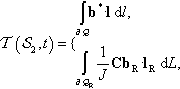
B(S2,t)={∫Qb*·nda,∫QRbR·NdA,E(S2,t)={∫∂Qe*·ldl,∫∂QReR·lRdL,

where dl and dL are line elements in the present and reference configurations, I and IR are unit tangents in the present and reference configurations, b* and bR are the spatial magnetic flux density and referential magnetic flux density (or magnetic induction), and e* and eR are the spatial electric field and referential electric field. Refer to Table 9.1 for their respective units. Use of (9.26) in (9.25) leads to Eulerian and Lagrangian representations of Faraday's law:
ddt∫Qb*·nda=−∫∂Qe*·ldl,

ddt∫QRbR·NdA=−∫∂QReR·lRdL.
Note that these integral statements are valid for any open surface Q![]() bounded by a closed curve ∂Q
bounded by a closed curve ∂Q![]() in the present configuration, or corresponding open surface QR
in the present configuration, or corresponding open surface QR![]() bounded by a closed curve ∂QR
bounded by a closed curve ∂QR![]() in the reference configuration.
in the reference configuration.
9.1.9 Gauss's law for magnetism
Gauss's law for magnetism (a statement of conservation of magnetic flux, or, alternatively, the absence of magnetic monopoles) postulates that the magnetic flux B![]() through any closed material surface is zero, i.e.,
through any closed material surface is zero, i.e.,
B(S1,t)=0.
Assuming that the magnetic flux B(S1,t)![]() through the surface of S1
through the surface of S1![]() (recall that S1
(recall that S1![]() consists of an open volume bounded by a closed surface) at time t is smooth, we can write
consists of an open volume bounded by a closed surface) at time t is smooth, we can write
B(S1,t)={∫∂Pb*·nda,∫∂PRbR·NdA.

Use of (9.29) in (9.28) gives Eulerian and Lagrangian representations of Gauss's law for magnetism:
∫∂Pb*·nda=0,

∫∂PRbR·NdA=0.

9.1.10 Gauss's law for electricity
Gauss's law for electricity postulates that the electric flux F![]() through any closed material surface is proportional to the total electric charge (i.e., free charge Σ plus bound charge Σb) enclosed within that surface, i.e.,
through any closed material surface is proportional to the total electric charge (i.e., free charge Σ plus bound charge Σb) enclosed within that surface, i.e.,
F(S1,t)=Σ(S1,t)+Σb(S1,t)εo,
where εo is the electric permittivity in vacuo. Assuming that the electric flux F![]() is smooth implies that
is smooth implies that
F(S1,t)={∫∂Pe*·nda,∫∂PRJC−1eR·NdA,

where J is the determinant of the deformation gradient F, and C−1 is the inverse of the right Cauchy-Green deformation tensor C = FTF. Recall that the free charge Σ and the bound charge Σb associated with subset S1![]() at time t are given in (9.22). Subsequent use of (9.22) and (9.32) in (9.31) leads to Eulerian and Lagrangian representations of Gauss's law for electricity:
at time t are given in (9.22). Subsequent use of (9.22) and (9.32) in (9.31) leads to Eulerian and Lagrangian representations of Gauss's law for electricity:
∫∂Pd*·nda=∫Pσ*dv,
∫∂PRdR·NdA=∫PRσRdV,

where the spatial electric displacement d* and referential electric displacement dR are introduced through the algebraic relationships (see, for instance, [37])
d*=p*+εoe*,dR=pR+εoJC−1eR.
9.1.11 Ampère-maxwell law
The Ampère-Maxwell law postulates that the time rate of change of the electric flux F![]() through any open material surface plus the conductive current J
through any open material surface plus the conductive current J![]() , polarization current Jp
, polarization current Jp![]() , and magnetization current Jm
, and magnetization current Jm![]() passing through that surface is proportional to the magnetic field T
passing through that surface is proportional to the magnetic field T![]() around the closed material curve bounding that surface. Application of this primitive statement of the law to subset S2
around the closed material curve bounding that surface. Application of this primitive statement of the law to subset S2![]() (an open material surface bounded by a closed material curve) allows us to express the Ampère-Maxwell law mathematically in material form:
(an open material surface bounded by a closed material curve) allows us to express the Ampère-Maxwell law mathematically in material form:
μo((εo)ddtF(S2,t)+J(S2,t)+Jp(S2,t)+Jm(S2,t))=T(S2,t),
where μo is the magnetic permeability in vacuo. Smoothness allows us to write
F(S2,t)={∫Qe*·nda,∫QRJC−1eR·NdA,J(S2,t)={∫Qj*·nda,∫QRjR·NdA,

Jp(S2,t)={ddt∫Qp*·nda,ddt∫QRpR·NdA,Jm(S2,t)={∫Q(curlm*)·nda,∫QR(CurlmR)·NdA,

T(S2,t)={∫∂Qb*·ldl,∫∂QR1JCbR·lRdL,
where m* and mR are the spatial magnetization and referential magnetization (or magnetic polarization), “curl” is the Eulerian curl (i.e., the curl calculated with respect to the present configuration), and “Curl” is the Lagrangian curl (i.e., the curl calculated with respect to the reference configuration). Use of (9.36)–(9.38) in (9.35) leads to
ddt∫Qd*·nda+∫Qj*·nda=∫∂Qh*·ldl,

ddt∫QRdR·NdA+∫QRjR·NdA=∫∂QRhR·lRdL,
where we have used (9.34) to introduce d* and dR, and the algebraic relationships (see, for instance, [36])
h*=1μob*−m*,hR=1μoJCbR−mR

to introduce the spatial magnetic field h* and referential magnetic field hR.
9.1.12 Transformations between spatial and referential TEMM quantities
The spatial (Eulerian) and referential (Lagrangian) TEMM quantities appearing in Sections 9.1.2–9.1.11, along with their corresponding units, are listed in Table 9.1. (In Table 9.1, we employ the following notation for the fundamental units: M is mass, LP is present length, LR is reference length, T is time, θ is temperature, and C is charge.)7 It can be shown that these spatial and referential quantities are related through the following linear algebraic transformations:
eR=FTe*,pR=JF−1p*,dR=JF−1d*,σR=Jσ*,hR=FTh*,mR=FTm*,bR=JF−1b*ρR=Jρ,jR=JF−1j*,P=JTF−T,qR=JF−1q.

Recall that J is the determinant of the deformation gradient F, and is a measure of dilatation or volume change (refer to Section 3.6). Several of these results—namely, (9.41)8, (9.41)10, and (9.41)11—were obtained in Sections 4.10 and 4.12. The other transformations can be obtained in a similar manner; refer to Problems 9.1–9.3.
Problem 9.1
Verify that eR = FTe*.
Recall from (9.26)2 that depending on whether we label the closed curve enclosing subset S2![]() by its present location ∂Q
by its present location ∂Q![]() or its reference location ∂QR
or its reference location ∂QR![]() , the electromotive force E
, the electromotive force E![]() induced in the boundary of S2
induced in the boundary of S2![]() has the following Eulerian and Lagrangian integral representations:
has the following Eulerian and Lagrangian integral representations:
E(S2,t)={∫∂Qe*·ldl,∫∂QReR·lRdL.

It follows that
∫∂Qe*·ldL=∫∂QReR·lRdL.

Upon a change of independent variable from x to X, the left-hand side of (a) becomes
∫∂Qe*·ldl=∫∂QReR·FlRdL,

where we have used
dl=FdlR,
i.e., the deformation gradient F linearly maps each line element dIR = IR dL in the reference configuration into a line element dI = I dl in the present configuration. (Refer to (3.28), and recall that IR and I are unit tangents in the reference and present configurations, and dL and dl are the infinitesimal lengths of the line elements.) Substitution of (b) into (a), and subsequent use of the definition (2.13) of the transpose of a tensor, leads to
∫∂QR(FTe*−eR)·lRdL=0.

Since the integrand is continuous and ∂QR![]() is arbitrary, the localization theorem in Section 4.5.2 implies that
is arbitrary, the localization theorem in Section 4.5.2 implies that
(FTe*−eR)·lR=0.
Since the coefficient of IR is independent of IR, and IR is arbitrary, it follows that
eR=FTe*.
An alternative proof that starts with the electric flux F![]() (refer to (9.32)) instead of the electromotive force E
(refer to (9.32)) instead of the electromotive force E![]() (refer to (9.26)2) is left as an exercise for the reader.
(refer to (9.26)2) is left as an exercise for the reader.
Problem 9.2
Verify that σR = Jσ*.
Recall from (9.22)1 that depending on whether we label the volume occupied by subset S1![]() by its present location P
by its present location P![]() or its reference location PR
or its reference location PR![]() , the free charge Σ within S1
, the free charge Σ within S1![]() has the following Eulerian and Lagrangian integral representations:
has the following Eulerian and Lagrangian integral representations:
Σ(S1,t)={∫Pσ*dv,∫PRσRdV.

It follows that
∫Pσ*dv=∫PRσRdV.

The left-hand side of (a), after a change of independent variable from x to X and use of the relationship dv = J dV (refer to (3.71)), becomes
∫Pσ*dv=∫PRσ*JdV.

Substitution of (b) into (a) and use of the localization theorem leads to
σR=Jσ*.
Problem 9.3
Verify that bR = JF−1b*.
Recall from (9.29) that depending on whether we label the closed surface bounding subset S1![]() by its present location ∂P
by its present location ∂P![]() or its reference location ∂PR
or its reference location ∂PR![]() , the magnetic flux B
, the magnetic flux B![]() through the boundary of S1
through the boundary of S1![]() has the following Eulerian and Lagrangian integral representations:
has the following Eulerian and Lagrangian integral representations:
B(S1,t)={∫∂Pb*·nda,∫∂PRbR·NdA.

It follows that
∫∂Pb*·nda=∫∂PRbR·NdA.

Upon a change of independent variable from X to x, the right-hand side of (a) becomes
∫∂PRbR·NdA=∫∂P1JbR·FTnda,

where we have used the relationship
JNdA=FTnda
from Section 3.6. Substitution of (b) into (a), and subsequent use of the definition (2.13) of the transpose of a tensor, leads to
∫∂P(b*−1JFbR)·nda=0.
The localization theorem then implies that
(b*−1JFbR)·n=0.

Since the coefficient of n is independent of n, and n is arbitrary, it follows that
bR=JF−1b*.
Note that this relationship can also be obtained starting from the Eulerian and Lagrangian integral representations of the magnetic field T![]() in (9.38), an exercise that we leave to the reader.
in (9.38), an exercise that we leave to the reader.
Exercises
1. Confirm that use of the free charge (9.22)1, bound charge (9.22)2, conductive current (9.23)1, and polarization current (9.23)2 in the material form of conservation of charge (9.21) leads to the integral forms (9.24a) and (9.24b).
2. Verify that use of the free charge (9.22)1, bound charge (9.22)2, and electric flux (9.32) in the material form of Gauss's law for electricity (9.31) leads to the integral forms (9.33a) and (9.33b).
3. Demonstrate that use of (9.36)–(9.38) in the material form of the Ampère-Maxwell law (9.35) leads to the integral forms (9.39a) and (9.39b). (Hint: You will need to use Stokes's theorem (9.44) to convert the magnetization current (9.37)2 from a surface integral to a line integral.)
4. Prove all transformations in (9.41) that remain unverified.
5. Using the fundamental units provided in Table 9.1, verify that the following equations are dimensionally homogeneous (i.e., all terms in the equation have the same units):
(a) The Eulerian and Lagrangian integral forms of the electromagnetic balance laws.
(b) The algebraic relationships (9.34) and (9.40).
(c) The transformations (9.41).
9.2 The fundamental laws of continuum electrodynamics: pointwise forms
In this section, we derive pointwise versions of the Eulerian and Lagrangian integral balance laws presented in Section 9.1.
9.2.1 Eulerian fundamental laws
We begin by recalling the Eulerian integral forms of the first principles developed in Section 9.1:
Conservation of mass
ddt∫Pρdv=0,

Balance of linear momentum
ddt∫Pvρdv=∫P(fm+fem)ρdv+∫∂Ptda,

Balance of angular momentum
ddt∫Px×vρdv=∫Px×(fm+fem)ρdv+∫∂Px×tda+∫Pcemρdv,

First law of thermodynamics
ddt∫P12v·vρdv+ddt∫Pερdv=∫P(fm+fem)·vρdv+∫∂Pt·vda+∫P(rt+rem)ρdv−∫∂Phda,

Second law of thermodynamics
ddt∫Pηρdv≥∫PrtΘρdv−∫∂PhΘda,

Conservation of electric charge
ddt∫Pσ*dv=−∫∂Pj*·nda,
Gauss's law for magnetism
∫∂Pb*·nda=0,

Faraday's law
ddt∫Qb*·nda=−∫∂Qe*·ldl,

Gauss's law for electricity
∫∂Pd*·nda=∫Pσ*dv,

Ampère-Maxwell law
ddt∫Qd*·nda+∫Qj*·nda=∫∂Qh*·ldl.
To obtain pointwise versions of the integral equations (9.42a)–(9.42j), we use tools similar to those employed in Section 4.8, including the transport theorem for volume integrals (refer to Section 4.5.1), the divergence theorem (refer to (2.104)), and the localization theorem (refer to Section 4.5.2). Several additional tools that will prove useful in this section include the transport theorem for surface integrals (refer to Problem 9.4)
ddt∫Qa·nda=∫Q[a′+curl(a×v)+v(diva)]·nda

and Stokes's theorem
∫∂Qa·ldl=∫Q(curla)·nda,

where a=˜a(x,t)![]() is an arbitrary vector-valued function of present position x and time t, v is the velocity, “div” denotes the Eulerian divergence (i.e., the divergence calculated with respect to the present configuration), “curl” denotes the Eulerian curl, and
is an arbitrary vector-valued function of present position x and time t, v is the velocity, “div” denotes the Eulerian divergence (i.e., the divergence calculated with respect to the present configuration), “curl” denotes the Eulerian curl, and
a′=∂∂t˜a(x,t)
denotes the Eulerian time derivative, i.e., the partial derivative of the spatial description of a with respect to time t. Also useful are the relations
t=Tn,h=q·n,
where T is the Cauchy stress and q is the spatial heat flux vector. Note that the proofs of (9.45)1 and (9.45)2 in a thermo-electro-magneto-mechanical setting are essentially identical to the corresponding proofs in a thermomechanical setting (refer to Section 4.6). With these tools in hand, it can be shown (refer, for instance, to Problem 9.5) that the pointwise variants of the Eulerian integral equations (9.42a)–(9.42j) are
˙ρ+ρdivv=0,
ρ˙v=ρ(fm+fem)+divT,
ρΓem+T−TT=0,
ρ˙ε=T·L+ρ(rt+rem)−divq,
ρ˙η≥ρrtΘ−div(qΘ),
˙σ*+σ*divv+divj*=0,
divb*=0,
curle*=−(b*)′−curl(b*×v),
divd*=σ*,
curlh*=(d*)′+curl(d*×v)+σ*v+j*,
where L = grad v is the Eulerian velocity gradient, Γem is a skew tensor whose corresponding axial vector is cem, i.e., Γema = cem × a for any vector a, and
˙a=a′+(v·grad)a
denotes the material time derivative of an arbitrary vector a=˜a(x,t)![]() . Note that in deriving the pointwise version of the first law of thermodynamics (9.46d) from its integral counterpart (9.42d), we have made use of the Eulerian form of the energy theorem for continuum electrodynamics:
. Note that in deriving the pointwise version of the first law of thermodynamics (9.46d) from its integral counterpart (9.42d), we have made use of the Eulerian form of the energy theorem for continuum electrodynamics:
∫P(fm+fem)·vρdv+∫∂Pt·vda−ddt∫P12v·vρdv=∫PT·Ldv.
Compare (9.47) with (4.33), the Eulerian form of the energy theorem for mechanics.