
Problem 9.4
Prove the transport theorem for surface integrals. That is, show that
ddt∫Qa·nda=∫Q[a′+curl(a×v)+v(diva)]·nda.
We begin by using relationship (3.76) between n da and N dA, together with a change of independent variable from x to X, to convert the Eulerian integration to a Lagrangian integration, i.e.,
ddt∫Qa·nda=ddt∫QRa·JF−TNdA.

We emphasize that the integrand on the left-hand side is a function of x and t, while the integrand on the right-hand side is a function of X and t. Then, it follows that
ddt∫Qa·nda=ddt∫QRJF−1a·NdA(definition(2.13))=∫QR·¯JF−1a·NdA(fixed region of integrationQR)=∫QR(˙JF−1a+J·¯F−1a+JF−1˙a)·NdA(product rule(3.22)).

We now individually examine the three terms on the right-hand side of the above equation. For the first term, we have
∫QR˙JF−1a·NdA=∫QRJ(divv)F−1a·NdA(result(3.60)3)=∫QRa(divv)·JF−TNdA(definition(2.13)).

For the second term, we have
∫QRJ·¯F−1a·NdA=−∫QRJF−1La·NdA(result(3.61)2)=−∫QRLa·JF−1NdA(definition(2.13))=−∫QR(gradv)a·JF−TNdA(definition(3.56)).

For the third term, we have
∫QRJF−1˙a·NdA=∫QR˙a·JF−TNdA(definition(2.13)).
Assembling the preceding results yields
ddt∫Qa·nda=∫QR(˙a+a(divv)−(gradv)a)·JF−TNdA.
We convert the Lagrangian integration to an Eulerian integration with a change of independent variable from X to x and use of the relationship (3.76) between N dA and n da:
ddt∫Qa·nda=∫Q(˙a+a(divv)−(gradv)a)·nda.

Use of results (2.102) and (3.20)2 leads to
ddt∫Qa·nda=∫Q(a′+curl(a×v)+v(diva))·nda.
Problem 9.5
Starting with the Eulerian (or spatial) statement of the Ampère-Maxwell law in integral form,
ddt∫Qd*·nda+∫Qj*·nda=∫∂Qh*·ldl,

derive the corresponding pointwise form
curlh*=(d*)′+curl(d*×v)+σ*v+j*.
We begin with the Eulerian integral form of the Ampère-Maxwell law, i.e.,
ddt∫Qd*·nda+∫Qj*·nda=∫∂Qh*·ldl.

We consider the first term on the left-hand side of (a):
ddt∫Qd*·nda=∫Q[(d*)′+curl(d*×v)+v(divd*)]·nda(transport theorem(9.43))=∫Q[(d*)′+curl(d*×v)+σ*v]·nda(Gauss's law(9.46i)).

Next, we consider the right-hand side of (a), which, after use of Stokes's theorem (9.44), becomes
∫∂Qh*·ldl=∫Q(curlh*)·nda.

Substitution of the preceding results into (a) leads to
∫Q[(d*)′+curl(d*×v)+σ*v+j*−curlh*]·nda=0.
Since the integrand is continuous and Q![]() is arbitrary, the localization theorem implies that
is arbitrary, the localization theorem implies that
[(d*)′+curl(d*×v)+σ*v+j*−curlh*]·n=0.
Furthermore, since the coefficient of n is independent of n, and n is arbitrary, it follows that the coefficient must vanish, i.e.,
curlh*=(d*)′+curl(d*×v)+σ*v+j*.
It is important to note that the electromagnetic equations (9.46f)–(9.46j) are not independent. For instance, it can be shown that conservation of charge (9.46f) is implicitly contained in Maxwell's equations (9.46g)–(9.46j); refer to Problem 9.6.
Problem 9.6
Show that conservation of charge (9.46f) is a consequence of Maxwell's equations (9.46g)–(9.46j).
Taking the divergence of the Ampère-Maxwell law (9.46j), and subsequently using result (2.101), gives
div[(d*)′]+div(σ*v)+divj*=0.
Continuity of d* enables the order of partial differentiation to be exchanged, so
div[(d*)′]=(divd*)′.
This, together with result (2.99)2, implies that
(divd*)′+v·gradσ*+σ*divv+divj*=0.
We then invoke Gauss's law for electricity (9.46i) and relationship (3.20)1 to recover
˙σ*+σ*divv+divj*=0,
the pointwise Eulerian statement of conservation of charge.
Exercises
2. Confirm that h = q · n.
3. Prove that (9.46a)–(9.46i) are the pointwise versions of the Eulerian integral forms of the fundamental laws (9.42a)–(9.42i).
9.2.2 Lagrangian fundamental laws
Recall from Section 9.1 the Lagrangian integral forms of the first principles:
Conservation of mass
∫Pρdv=∫PRρRdV,
Balance of linear momentum
ddt∫PRvρRdV=∫PR(fm+fem)ρRdV+∫∂PRtRdA,

Balance of angular momentum
ddt∫PRx×vρRdV=∫PRx×(fm+fem)ρRdV+∫∂PRx×tRdA+∫PRcemρRdV,

First law of thermodynamics
ddt∫PR12v·vρRdV+ddt∫PRερRdV=∫PR(fm+fem)·vρRdV+∫∂PRtR·vdA+∫PR(rt+rem)ρRdV−∫∂PRhRdA,

Second law of thermodynamics
ddt∫PRηρRdV≥∫PRrtΘρRdV−∫∂PRhRΘdA,
Conservation of electric charge
ddt∫PRσRdV=−∫∂PRjR·NdA,

Gauss's law for magnetism
∫∂PRbR·NdA=0,

Faraday's law
ddt∫QRbR·NdA=−∫∂QReR·lRdL,
Gauss's law for electricity
∫∂PRdR·NdA=−∫PRσRdV,
Ampère-Maxwell law
ddt∫QRdR·NdA+∫QRjR·NdA=∫∂QRhR·lRdL.

An important feature of the Lagrangian integral conservation laws (9.48a)–(9.48j) is that the regions PR![]() and QR
and QR![]() occupied by subsets S1
occupied by subsets S1![]() and S2
and S2![]() in the reference configuration are fixed. Hence, the regions of integration PR
in the reference configuration are fixed. Hence, the regions of integration PR![]() and QR
and QR![]() do not change with time, so time derivatives of Lagrangian surface and volume integrals can be passed directly inside the integrals. Conversely, with the Eulerian integral conservation laws (9.42a)–(9.42j), the regions of integration P
do not change with time, so time derivatives of Lagrangian surface and volume integrals can be passed directly inside the integrals. Conversely, with the Eulerian integral conservation laws (9.42a)–(9.42j), the regions of integration P![]() and Q
and Q![]() change with time. Thus, to take time derivatives of these time-varying integrals, the transport theorem for surface integrals (9.43) and the transport theorem for volume integrals (4.20) must be employed. The transport theorems are analogous to Leibniz's rule in multivariable calculus.
change with time. Thus, to take time derivatives of these time-varying integrals, the transport theorem for surface integrals (9.43) and the transport theorem for volume integrals (4.20) must be employed. The transport theorems are analogous to Leibniz's rule in multivariable calculus.
The continuous, bounded nature of the integrands in (9.48a)–(9.48j) enables the divergence theorem and Stokes's theorem, and the requirement that (9.48a)–(9.48j) be continuous and global, i.e., true for the entire body and all subsets, enables the localization theorem. With the traction tR and heat flux hR dependent on surface geometry only through the outward unit normal N, so tR = PN and hR = qR · N, it can be shown that application of the divergence theorem, Stokes's theorem, and the localization theorem to the Lagrangian integral equations (9.48a)–(9.48j) leads to the Lagrangian pointwise equations
ρJ=ρR,
ρR˙v=ρR(fm+fem)+DivP,
ρRΓem+PFT−FPT=0,
ρR˙ε=P·Gradv+ρR(rt+rem)−DivqR,
ρR˙η≥ρRrtΘ−Div(qRΘ),

˙σR+DivjR=0,
DivbR=0,
CurleR=−˙bR,
DivdR=σR,
CurlhR=˙dR+jR.
Note that it can be shown that conservation of charge (9.49f) is not independent of Maxwell's equations(9.49g)–(9.49j), but rather is implicitly contained in them. Recall that P is the first Piola-Kirchhoff stress, qR is the referential heat flux vector, “Div” is the Lagrangian divergence (i.e., the divergence calculated with respect to the reference configuration), “Curl” is the Lagrangian curl, and
˙a=∂∂tˆa(X,t)
is the material derivative of an arbitrary vector a=ˆa(X,t)![]() , i.e., the partial derivative of the referential description of a with respect to time t. Also,
, i.e., the partial derivative of the referential description of a with respect to time t. Also,
Γema=cem×a
for any vector a, i.e., Γem is a skew tensor whose corresponding axial vector is cem. Note that in deriving the pointwise version of the first law of thermodynamics (9.49d) from its integral counterpart (9.48d), we have made use of the Lagrangian form of the energy theorem for continuum electrodynamics:
∫PR(fm+fem)·vρRdV+∫∂PRtR·vdA−ddt∫PR12v·vρRdV=∫PRP·GradvdV.

Compare (9.50) with (4.54), the Lagrangian form of the energy theorem for mechanics.
Exercises
2. Confirm that hR = qR · N.
3. Prove that (9.49a)–(9.49j) are the pointwise versions of the Lagrangian integral forms of the fundamental laws (9.48a)–(9.48j).
4. Show that conservation of charge (9.49f) is a consequence of Maxwell's equations (9.49g)–(9.49j).
9.3 Modeling of the effective electromagnetic fields
Recall that Eulerian modeling of deformable thermo-electro-magneto-mechanical materials involves two sets of spatial (or Eulerian) electromagnetic fields: the effective fields e*, d*, p*, h*, b*, m*, σ*, and j*, distinguished in our notation by superscript asterisks, and the standard fields e, d, p, h, b, m, σ, and j. (Conversely, in Lagrangian modeling, there is no notion of effective or standard fields.) The effective fields are the electromagnetic fields acting on the deforming continuum as seen in its present configuration, measured with respect to a co-moving or rest frame, i.e., a frame affixed to but not deforming with the continuum. The standard fields also act on the deforming continuum as seen in its present configuration, but are instead measured with respect to a fixed or laboratory frame.
Various transformations have been presented in the literature that relate the effective fields to the standard fields.8 In this section, we present four popular transformation theories, each based on a different set of principles and postulates. As a result, the standard electromagnetic fields generally have different physical connotations from model to model; hence, in what follows, the fields corresponding to a particular model are distinguished with the appropriate subscript notation.
9.3.1 Minkowski model
The Minkowski model [32, 33, 38] is motivated by Einstein's special theory of relativity. In this approximation, the effective fields are related to the standard fields through semirelativistic inverse Lorentz transformations:
e*=eM+v×bM,h*=hM−v×dM,d*=dM,b*=bM,p*=pM,m*=mM+v×pM,j=jM−σMv,σ*=σM,

where (·)M represents a standard electromagnetic field corresponding to the Minkowski model.
9.3.2 Lorentz model
The Lorentz model is motivated by Lorentz's theory of electrons [39], which postulates that a body consists of an infinitely large number of rapidly moving charged particles. The motion of these charged particles, in turn, generates rapidly fluctuating microscopic electromagnetic fields. The microscopic fields averaged over a small time interval and an infinitesimal volume are defined as the corresponding macroscopic fields. The aforementioned postulates lead to the following relationships:
e*=eL+v×bL,h*=hL−∈ov×eL,d*=dL,b*=bL,p*=pL,m*=mL,j*=jL−σLv,σ*=σL,

where (·)L represents a standard electromagnetic field corresponding to the Lorentz model.
9.3.3 Statistical model
The statistical model [40] is a modification of Lorentz's theory, wherein the charged particles are grouped into stable structures (e.g., atoms, molecules, or ions). The field effects of the charged particles within each stable structure are represented by microscopic electric and magnetic multipole moments (e.g., dipole, quadrupole, and octupole moments), and the macroscopic polarization and magnetization fields are defined as statistical averages of these multipole moments over a large number of stable structures. The transformations presented in this model are identical to Minkowski's, i.e.,
e*=eS+v×bS,h*=hS−v×dS,d*=dS,b*=bS,p*=pS,m*=mS+v×pS,j*=jS−σSv,σ*=σS,

where ( )s represents a standard electromagnetic field corresponding to the statistical model.
9.3.4 CHU model
The Chu model [41] is based on the postulate that deforming bodies contribute to electromagnetic phenomena by acting, in a macroscopic sense, as electric and magnetic dipole sources for the electromagnetic fields. The transformations for the Chu model are
e*=eC+μO×hC,h*=hC−∈ov×eC,d*=dC,b*=bC,p*=pC+mC×vc2,m*=mC,j*=jC−σCv,σ*=σC,

where ( )c represents a standard electromagnetic field corresponding to the Chu model.
9.3.5 A comparison of the four models
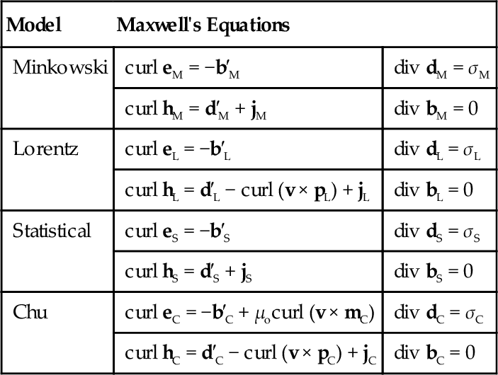
Table 9.2 catalogs Maxwell's equations for each of the four models, deduced by substituting each set of transformations (i.e., (9.51)–(9.54)) into (9.46g)–(9.46j). Recall that since each of the four models is based on a different set of postulates, the standard electromagnetic fields generally have different physical connotations from model to model. We can deduce relationships between the standard fields by comparing the equations in Table 9.2. For instance, the Minkowski and statistical models, although developed from different perspectives, are mathematically equivalent (i.e., mM = ms, pM = ps, etc.).
Table 9.2
Maxwell's Equations for Different Transformation Models
| Model | Maxwell's Equations | |
| Minkowski | curl eM = −b′M | div dM = σM |
| curl hM = d′M + jM | div bM = 0 | |
| Lorentz | curl eL = −b′L | div dL = σL |
| curl hL = d′L − curl (v × pL) + jL | div bL = 0 | |
| Statistical | curl eS = −b′S | div dS = σS |
| curl hS = d′S + jS | div bS = 0 | |
| Chu | curl eC = −b′C + μocurl (v × mC) | div dC = σC |
| curl hC = d′C − curl (v × pC) + jC | div bC = 0 | |
Problem 9.7
Verify the results presented in Table 9.2 for the Minkowski model.
Straightforward substitution of the Minkowski transformations (9.51)3, (9.51)4, and (9.51)8 into the Eulerian forms of Gauss's law for magnetism (9.46g) and Gauss's law for electricity (9.46i) gives
divbM=0,divdM=σM.
Then, use of the transformation equations (9.51)2, (9.51)3, (9.51)7, and (9.51)8, i.e.,
h*=hM−v×dM,d*=dM,j*=jM−σMv,σ*=σM,
in the Ampère-Maxwell law (9.46j) leads to
curl(hM−v×dM)=d′M+curl(dM×v)+σMv+(jM−σMv).
Anticommutativity of the vector product (2.61) and the distributive property of the curl (2.103a) then imply that the above equation becomes
curlhM=d′M+jM.
Similarly, Faraday's law (9.46h) is transformed by applying (9.51)1 and (9.51)4:
curl(eM+v×bM)=−b′M−curl(bM×v).
Simplification of this result using (2.61) and (2.103a) leads to
curleM=−b′M.
Exercise
1. Verify the results presented in Table 9.2 for the Lorentz, statistical, and chu models.
9.4 Modeling of the electromagnetically induced coupling terms
As discussed in Section 9.1, the thermomechanical equations ((9.46a)–(9.46d) in Eulerian form) are coupled to the electromagnetic equations ((9.46f)–(9.46j) in Eulerian form) through the electromagnetic body force fem, body couple cem (or, equivalently, Γem), and energy supply rate rem. The mathematical forms of these coupling terms are postulated on the basis of the interaction theories presented in Section 9.3, which are motivated by either atomic physics or empiricism. As an example, the coupling terms postulated using the Minkowski theory for apolarizable, magnetizable, deformable continuum are, in Eulerian form [32],
ρfem=σ*e*+j*×b*+(grade*)Tp*+μo(gradh*)Tm*+∘d*×b*+d*×∘b*,
ρΓem=(e*⊗p*−p*⊗e*)+μo(h*⊗m*−m*⊗h*),
ρrem=j*·e*+ρe*··¯(p*ρ)+ρμoh*··¯(m*ρ),

where we recall that () ⊗ () denotes the dyadic product of two vectors, “grad” is the Eulerian gradient, and
å=a′+curl(a×v)+v(diva)
is a convected rate of an arbitrary vector a=˜a(x,t)![]() . coupling terms for the Lagrangian forms of the fundamental laws can be found, for instance, in [32].
. coupling terms for the Lagrangian forms of the fundamental laws can be found, for instance, in [32].
The Minkowski model (9.55a)–(9.55c) has as special cases interaction theories describing forces exerted by static electric fields in polarizable solids [42] and static magnetic fields in magnetizable solids [43]. Use of (9.55a)–(9.55c) in the Eulerian forms of balance of linear momentum (9.46b), balance of angular momentum (9.46c), and the first law of thermodynamics (9.46d) yields
ρ˙v=ρfm+σ*e*+j*×b*+(grade*)Tp*+μo(gradh*)Tm*+∘d*×b*+d*×∘b*+divT,
T−TT=(p*⊗e*−e*⊗p*)+μo(m*⊗h*−h*⊗m*),
˙ε=1ρRP·˙F+e*··¯(p*ρ)+μoh*··¯(m*ρ)+rt+1ρj*·e*−1ρdivq.

9.4.1 An alternative approach
Electromagnetic effects in the thermomechanical balance laws can be modeled as an electromagnetically induced body force, body couple, and energy supply (as discussed previously; see also [32, 33, 44]) or, alternatively, incorporated into the constitutive response (see, for instance, [34–36]). The latter is accomplished by defining a symmetrictotal stress tensor
τ=T+Tem
that consists of contributions from the cauchy stress tensor T and the electromagnetic Maxwell stress tensor Tem. The Maxwell stress Tem is defined so that twice its skew part is ρΓem and its divergence is ρfem; refer to Problem 9.8. For the Minkowski formulation (9.55a)–(9.55c), it can be shown that
Tem=e*⊗d*+h*⊗b*−12(εoe*·e*+μoh*·h*)I.
By formulating the first principles and the constitutive equations in terms of the total stress τ instead of the Cauchy stress T, we eliminate explicit coupling between the electromagnetic fields and the thermomechanical fields in the first principles (9.57a)–(9.57c). This coupling is instead accounted for implicitly through the constitutive equation for τ.
Problem 9.8
Prove that the divergence of the Maxwell stress tensor Tem in (9.59) is equal to the electromagnetic body force vector ρfem in (9.55a).
Taking the divergence of the Maxwell stress tensor (9.59) gives
divTem=div[e*⊗d*+h*⊗b*−12(εoe*·e*+μoh*·h*)I].

The divergence is distributive over tensor addition (refer to (2.103b)), which implies that
divTem=div(e*⊗d*)+div(h*⊗b*)=12{εodiv[(e*·e*)I]+μodiv[(h*·h*)I]}.
The first term in (a) simplifies to
div(e*⊗d*)=(divd*)e*+(grade*)d*(result(2.99)7)=σ*e*+(grade*)d*(Gauss's law(9.46i)).

Similarly, the second term reduces to
div(h*⊗b*)=(divb*)h*+(gradh*)b*(result(2.99)7)=(gradh*)b*(Gauss's law(9.46g)).

The third term in (a) simplifies to
12εodiv[(e*·e*)I]=12εograd(e*·e*)(result(2.99)6)=εo(grade*)Te*(result(2.99)3).
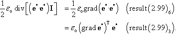
Similarly, use of results (2.99)3 and (2.99)6 reduces the fourth term to
12μodiv[(h*·h*)I]=μo(gradh*)Th*.
Combining results (b)–(e) in (a), we obtain
divTem=σ*e*+(grade*)d*+(gradh*)b*=[εo(grade*)Te*+μo(gradh*)Th*].
Relationships (9.34)1 and (9.40)1, i.e.,
d*=p*+εoe*,b*=μo(h*+m*),
allow us to rewrite (f) as
divTem=σ*e*+[grade*−(grade*)T]d*+[gradh*=(gradh*)T]b*+(grade*)Tp*+μo(gradh*)Tm*.
Invoking definition (2.100) of the curl implies that
divTem=σ*e*+(curle*)×d*+(curlh*)×b*+(grade*)Tp*+μo(gradh*)Tm*.
Faraday's law (9.46h) and the Ampère-Maxwell law (9.46j), i.e.,
curle*=−(b*)′−curl(b*×v),curlh*=(d*)′+curl(d*×v)+σ*v+j*,
are then used in (g), which, noting anticommutativity of the vector product, leads to
divTem=σ*e*+j*×b*+(grade*)Tp*+μo(gradh*)Tm*+[(d*)′+curl(d*×v)+σ*v]×b*+d*×[(b*)′+curl(b*×v)]
It then follows that
divTem=σ*e*+j*×b*+(grade*)Tp*+μo(gradh*)Tm*+∘d*×b*+d*×∘b*=ρfem,
where ∘b*![]() and ∘d*
and ∘d*![]() represent convected rates as defined in (9.56).
represent convected rates as defined in (9.56).
Exercises
2. Verify that use of the electromagnetic energy (9.55c) in the Eulerian form of the first law of thermodynamics (9.46d) leads to (9.57c).
3. Verify that
(a) twice the skew part of the Maxwell stress tensor Tem in (9.59) is ρΓem in (9.55b), and
(b) the total stress tensor τ in (9.58) is symmetric.
9.5 Thermo-electro-magneto-mechanical process
The pointwise Eulerian field equations (9.46a), (9.46f)–(9.46j), and (9.57a)–(9.57c) constitute the first principles of our model, true for all thermo-electro-magneto-mechanical (TEMM) materials. For the purposes of developing the constitutive equations that supplement these first principles and characterize particular TEMM materials, we conceptually divide the fields appearing in (9.46a), (9.46f)–(9.46j), and (9.57a)–(9.57c) into three groups:
{x,η,p*,m*},{P,Θ,e*,h*,ε,q,j*},{ρ,fm,rt,σ*},
denoted the independent variables, dependent variables, and balancing terms, respectively.9 (Note that the set of independent variables contains slots occupied by one mechanical, one thermal, one electrical, and one magnetic quantity, respectively, from left to right.) Hence, the first Piola-Kirchhoff stress P, temperature Θ, electric field e*, magnetic field h*, internal energy ε, heat flux q, and conductive current j* are determined from constitutive equations that, in general, depend on the history of the motion x, entropy η, electric polarization p*, and magnetization m*, and possibly their rates or gradients. A group of quantities x, η, p*, m*, P, Θ, e*, h*, ε, q, j*, ρ, fm, rt, and σ* that satisfy the governing equations (9.46a), (9.46f)–(9.46j), and (9.57a)–(9.57c) for all space and time in the domain of interest describes a TEMM process.
9.6 Constitutive model development for thermo-electro-magneto-elastic materials: large-deformation theory
In this section, we specialize to (1) thermo-electro-magneto-elastic (TEME) materials that are capable of undergoing large elastic strains before yielding and (2) material response that is reversible (i.e., path independent and rate insensitive). We then illustrate the development of a general finite-deformation TEME constitutive framework using the principles of continuum thermodynamics, and show how this framework can be simplified using restrictions imposed by the second law of thermodynamics, invariance, angular momentum, and material symmetry. Similar approaches have been used to develop constitutive models for particular classes of smart materials in the finite-deformation regime, e.g., electroactive elastomers and magnetosensitive elastomers; see, for instance, [35–37,45–60,]. The large-deformation constitutive framework presented in this section, on the other hand, is intended to model a more general range of smart material behavior (e.g., magneto-electric coupling).
9.6.1 The reduced clausius-duhem inequality, work conjugates
We algebraically combine the Eulerian forms of the Clausius-Duhem inequality (9.46e) and the first law of thermodynamics (9.57c) to produce the reduced Clausius-Duhem inequality
−˙ε+1ρRP·˙F+Θ˙η+e*··¯(p*ρ)+μoh*··¯(m*ρ)+1ρj*·e*−1ρΘq·gradΘ≥0.

Analogously to classical thermodynamics [61], this fundamental statement of the second law consists of contributions from conjugate pairs of thermal, electrical, magnetic, and mechanical quantities. Each of these conjugate pairs (or work conjugates) is the product of the rate of an extensive quantity in rate form (˙F![]() , ˙η
, ˙η![]() , (˙p*/ρ)
, (˙p*/ρ)![]() , and (˙m*/ρ)
, and (˙m*/ρ)![]() ) and an intensive quantity (P, Θ, e*, and h*).10 The utility of the second law, and our identification of the extensive and intensive quantities, will become apparent in the following section.
) and an intensive quantity (P, Θ, e*, and h*).10 The utility of the second law, and our identification of the extensive and intensive quantities, will become apparent in the following section.
Exercise
1. Verify that the Clausius-Duhem inequality (9.46e) can be algebraically combined with the first law of thermodynamics (9.57c) to produce the reduced Clausius-Duhem inequality (9.61).
9.6.2 The all-extensive formulation
Recall that we specialized to reversible TEME material response, which implies that the deformation, although it may be large, is elastic and fully recoverable, and the material only undergoes nondissipative TEMM processes. It follows, then, that these TEMM processes can be completely described through the principles of classical equilibrium thermodynamics11 [61].
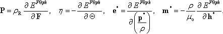
Analogously to classical equilibrium thermodynamics, our fundamental energy potential is the specific internal energy ε, which employs extensive quantities as its independent variables [61]. Hence, for the fundamental formulation, the natural independent variables are the extensive quantities F, η, p*/ρ, and m*/ρ appearing as rates in (9.61), and the natural dependent variables are the conjugate intensive quantities P, Θ, e*, and h*. Thus, for thermodynamic consistency, and to respect the reversible elastic nature of the process, we adjust the division (9.60) so that the dependence of the response on the present position x, polarization p*, and magnetization m* is through the deformation gradient F = Grad x, p*/ρ, and m*/ρ, respectively. Additionally, we demand that the response depends on these independent variables only through their values at the present time t, not their histories, rates, or gradients, i.e.,
P=˘P(F,η,p*ρ,m*ρ),Θ=˘Θ(F,η,p*ρ,m*ρ),e*=˘e*(F,η,p*ρ,m*ρ),h*=˘h*(F,η,p*ρ,m*ρ),ε=˘ε(F,η,p*ρ,m*ρ).
Notation (9.62) indicates that P, Θ, e*, h*, and ε are explicit functions of F, η, p*/p, and m*/ρ evaluated at present position x and time t, and implicit functions of x and t. Note that a superscript breve is used to distinguish a function from its value (or output). As with all materials in the TEMM theory, the response functions (9.62) for a TEME material must satisfy the second law of thermodynamics, invariance requirements, conservation of angular momentum, and material symmetry conditions.
In what follows, we demonstrate how restrictions imposed by the second law of thermodynamics (9.61) yield a set of constitutive equations that provide the dependent variables P, Θ, e*, and h* (the intensive quantities) as partial derivatives of the specific internal energy ε (the fundamental thermodynamic energy potential) with respect to the independent variables F, η, p*/ρ, and m*/ρ (the extensive quantities), respectively. Use of the chain rule on ε=˘ε(F,η,p*/ρ,m*/ρ)![]() gives
gives
˙ε=∂˘ε∂F·˙F+∂˘ε∂η˙η+∂˘ε∂(p*ρ)··¯(p*ρ)+∂˘ε∂(m*ρ)··¯(m*ρ),
and substitution of this result into the second law (9.61) leads to
(1ρRP−∂˘ε∂F)·˙F+(Θ−∂˘ε∂η)˙η+(e*−∂˘ε∂(p*ρ))··¯(p*ρ)+(μoh*−∂˘ε∂(m*ρ))··¯(m*ρ)+1ρj*·e*−1ρΘq·gradΘ≥0.

Inequality (9.63) must hold for all processes. Since the coefficients of the rates (˙F![]() , ˙η
, ˙η![]() , etc.) in (9.63) are independent of the rates themselves, and the rates may be varied independently and are arbitrary, it follows that the coefficients vanish, i.e.,
, etc.) in (9.63) are independent of the rates themselves, and the rates may be varied independently and are arbitrary, it follows that the coefficients vanish, i.e.,
P=ρR∂˘ε∂F,Θ=∂˘ε∂η,e*=∂˘ε∂(p*ρ),h*=1μo∂˘ε∂(m*ρ).

What remains of inequality (9.63), i.e.,
j*·e*−1Θq·gradΘ≥0,
is called the residual dissipation inequality. The residual dissipation inequality quantifies irreversibilities in a thermodynamic process. In this case, the first term in (9.65) represents Joule heating due to current flow, and the second term represents heat conduction; both are transport processes. Accordingly, unlike the other dependent variables (see (9.64)), the conductive current j* and heat flux q are not derivable from a thermodynamic energy potential. Instead, their constitutive equations are specified empirically (e.g., Ohm's law for j* and Fourier's law for q), with the caveat that they must satisfy inequality (9.65).
We collectively coin the set of extensive independent variables {F, η, p*/ρ, m*/ρ}, the thermodynamic energy potential {F,η,p*/ρ,m*/ρ}![]() , and the constitutive equations (9.64) the all-extensive formulation. The all-extensive formulation, along with the other formulations that we present in this section, correlate with a particular experiment, the independent variables being controlled and the dependent variables being the measured responses.
, and the constitutive equations (9.64) the all-extensive formulation. The all-extensive formulation, along with the other formulations that we present in this section, correlate with a particular experiment, the independent variables being controlled and the dependent variables being the measured responses.
9.6.2.1 Polarization and magnetization as independent variables
From an experimental point of view, it is more practical to control the electric polarization p* and magnetization m* than the polarization per unit mass p*/ρ and magnetization per unit mass m*/ρ. Hence, we modify the all-extensive formulation presented in Section 9.6.2 to accommodate the use of p* and m* as independent variables. We proceed by using the chain rule
·¯(p*ρ)=1ρ˙p*+1ρ(F−T·˙F)p*,·¯(m*ρ)=1ρ˙m*+1ρ(F−T·˙F)m*

to rewrite the fundamental form (9.61) of the Clausius-Duhem inequality:
−˙ε+[1ρRP+1ρ(e*·p*+μoh*·m*)F−T]·˙F+Θ˙η+1ρe*·˙p*+μoρh*·˙m*+1ρj*·e*−1ρΘq·gradΘ≥0,

where we have used
·¯(1ρ)=1ρdivv,divv=trL=tr(˙FF−1)=F−T·˙F.

In the modified form (9.67) of the second law, polarization p* and magnetization m* appear as rates (i.e., natural independent variables). Accordingly, the thermodynamic energy potential ε in this formulation is a function of F, η, p*, and m*, i.e., ε=ˉε(F,η,p*,m*)![]() ; a superscript bar is used instead of a superscript breve to signify a different internal energy function with the same value. Use of the chain rule gives
; a superscript bar is used instead of a superscript breve to signify a different internal energy function with the same value. Use of the chain rule gives
˙ε=∂ˉε∂F·˙F+∂ˉε∂η˙η+∂ˉε∂p*·˙p*+∂ˉε∂m*·˙m*,
and substitution of this result into (9.67) leads to
(1ρRP+1ρ(e*·p*+μoh*·m*)F−T−∂ˉε∂F)·˙F+(Θ−∂ˉε∂η)˙η+(1ρe*−∂ˉε∂p*)·˙p*+(μoρh*−∂ˉε∂m*)·˙m*+1ρj*·e*−1ρΘq·gradΘ≥0.

Since the coefficients of ˙F![]() , ˙η
, ˙η![]() , ˙p*
, ˙p*![]() , and ˙m*
, and ˙m*![]() in inequality (9.69) are independent of the rates, and the rates may be varied independently and are arbitrary, it follows that the coefficients vanish, i.e.,
in inequality (9.69) are independent of the rates, and the rates may be varied independently and are arbitrary, it follows that the coefficients vanish, i.e.,
P=ρR∂ˉε∂F−J(e*·p*+μoh*·m*)F−T,Θ=∂ˉε∂η,e*=ρ∂ˉε∂p*,h*=ρμo∂ˉε∂m*.
We collectively coin the set of independent variables {F, η, p*, m*}, the thermodynamic energy potential ε=ˉε(F,η,p*,m*)![]() , and the constitutive equations (9.70) the deformation-entropy-polarization-magnetization formulation.
, and the constitutive equations (9.70) the deformation-entropy-polarization-magnetization formulation.
Exercise
1. Verify the relationships in (9.68).
9.6.3 Other formulations
Knowledge of the internal energy function ε=˘ε(F,η,p*/ρ,m*/ρ)![]() or ε=ˉε(F,η,p*,m*)
or ε=ˉε(F,η,p*,m*)![]() is sufficient to characterize a reversible TEME material. Said differently, specifying the functional form of the energy potential determines P, Θ, e*, and h* in (9.64) and (9.70). The functional form of the energy potential is ascertained experimentally; this experimental characterization most straightforwardly accomplished when the independent and dependent variables synchronize with those one wishes to control and measure, respectively, in an experiment. From an experimental perspective, it is often more practical to control intensive quantities than extensive quantities; e.g., temperature is easier to control than entropy or internal energy. To change an independent variable from extensive to intensive, a new free energy is defined through a Legendre transformation of the internal energy, i.e.,
is sufficient to characterize a reversible TEME material. Said differently, specifying the functional form of the energy potential determines P, Θ, e*, and h* in (9.64) and (9.70). The functional form of the energy potential is ascertained experimentally; this experimental characterization most straightforwardly accomplished when the independent and dependent variables synchronize with those one wishes to control and measure, respectively, in an experiment. From an experimental perspective, it is often more practical to control intensive quantities than extensive quantities; e.g., temperature is easier to control than entropy or internal energy. To change an independent variable from extensive to intensive, a new free energy is defined through a Legendre transformation of the internal energy, i.e.,
new free energy=internal energy−(intensive)(extensive).
Following this blueprint, we present in Tables 9.3–9.6 a catalogue of the 15 possible Legendre transformations of the internal energy. These Legendre transformations are divided into four families, each employing a common set of thermomechanical independent variables: family 1, deformation and entropy (both extensive); family 2, deformation (extensive) and temperature (intensive); family 3, stress (intensive) and entropy (extensive); and family 4, stress and temperature (both intensive). For the sake of brevity, we employ the compact notation Eabcd for the Legendre-transformed energy potentials, where the superscript letters a, b, c, and d are placeholders for an appropriate mechanical, thermal, electrical, and magnetic independent variable, respectively. This compact notation denotes that the Legendre-transformed energy potential EFΘpm, for instance, is a function of deformation F, temperature Θ, electric polarization per unit mass p*/ρ, and magnetization per unit mass m*/ρ. Note that the Legendre transformations in Tables 9.3–9.6 provide explicit connections between the new free energies Eabcd and the primitive internal energy ε of the system, whose evolution is governed by the first law of thermodynamics (9.57c).
Table 9.3
Energy Family 1
| Independent Variables | Energy | Legendre Transformation |
| F, η, p*/ρ, m*/ρ | ε | |
| F, η, e*, m*/ρ | EFηem | EFηem=ε−e*·p*ρ |
| F, η, p*/ρ, h* | EFηph | EFηph=ε−μoh*·m*ρ |
| F, η, e*, h* | EFηeh | EFηeh=ε−e*·p*ρ−μoh*·m*ρ |
Table 9.4
Energy Family 2
| Independent Variables | Energy | Legendre Transformation |
| F, Θ, p*/ρ, m*/ρ | EFΘpm | EFΘpm = ε − Θη |
| F, Θ, e*, m*/ρ | EFΘem | EFΘem=ε−Θη−e*·p*ρ |
| F, Θ, p*/ρ, h* | EFΘph | EFΘph=ε−Θη−μoh*·m*ρ |
| F, Θ, e*, h* | EFΘeh | EFΘeh=ε−Θη−e*·p*ρ−μoh*·m*ρ |
Table 9.5
Energy Family 3
| Independent Variables | Energy | Legendre Transformation |
| P, η, p*/ρ, m*/ρ | EPηpm | EPηpm=ε−1ρRP·F |
| P, η, e*, m*/ρ | EPηem | EPηem=ε−1ρRP·F−e*·p*ρ |
| P, η, p*/ρ, h* | EPηph | EPηph=ε−1ρRP·F−μoh*·m*ρ |
| P, η, e*, h* | EPηeh | EPηeh=ε−1ρRP·F−e*·p*ρ−μoh*·m*ρ |
Table 9.6
Energy Family 4
| Independent Variables | Energy | Legendre Transformation |
| P, Θ, p*/ρ, m*/ρ | EPΘpm | EPΘpm=ε−1ρRP·F−Θη |
| P, Θ, e*, m*/ρ | EPΘem | EPΘem=ε−1ρRP·F−Θη−e*·p*ρ |
| P, Θ, p*/ρ, h* | EPΘph | EPΘph=ε−1ρRP·F−Θη−μoh*·m*ρ |
| P, Θ, e*, h* | EPΘeh | EPΘeh=ε−1ρRP·F−Θη−e*·p*ρ−μoh*·m*ρ |
The constitutive equations associated with the 15 formulations shown in Tables 9.3–9.6 are obtained via restrictions imposed by the second law of thermodynamics, invariance requirements, conservation of angular momentum, and material symmetry; refer to [62] for a complete catalogue. In the following sections, as a representative example, we investigate the deformation-temperature-electric field-magnetic field formulation. However, before we proceed, note the following:
(1) A procedure for introducing free energies that use the electric displacement d* and magnetic induction b* as independent variables, and the derivation of their associated constitutive equations, is presented in Appendix F.
(2) For formulations that employ either the electric polarization per unit mass p*/ρ or the magnetization per unit mass m*/ρ as an independent variable, as was the case with the all-extensive formulation in Section 9.6.2, p* or m* can be introduced as the independent variable ex post facto using the procedure described in Section 9.6.2.1. Refer to Problem 9.9.
Problem 9.9
Using the second law of thermodynamics and the appropriate Legendre transformation, derive the constitutive equations for the deformation-temperature-polarization-magnetic field formulation.
In this formulation, F, Θ, p*/ρ, and h* are the independent variables. We define the energy potential EFΘph as the Legendre transformation of internal energy ε=˘ε(F,η,p*/ρ,m*/ρ)![]() with respect to the thermal and magnetic variables, from η to Θ and m*/ρ to h*, i.e.,
with respect to the thermal and magnetic variables, from η to Θ and m*/ρ to h*, i.e.,
EFΘph=ε−Θη−μoh*·m*ρ.
Refer to Table 9.4. The rate of the Legendre transformation is
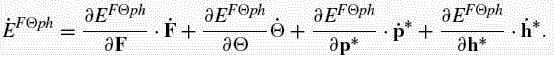
˙EFΘph=˙ε−Θ˙η−η˙Θ−μoh*··¯(m*ρ)−μom*ρ·˙h*,

and subsequent use of this result in the second law of thermodynamics (9.61) leads to
−˙EFΘph+1ρRP·˙F−η˙Θ+e*··¯(p*ρ)−μom*ρ·˙h*+1ρj*·e*−1ρΘq·gradΘ≥0.

Use of the chain rule on ˙EFΘph![]() gives
gives
˙EFΘph=∂EFΘph∂F·˙F+∂EFΘph∂Θ˙Θ+∂EFΘph∂(p*ρ)··¯(p*ρ)+∂EFΘph∂h*·˙h*,

and substitution of this result into inequality (a) leads to the constitutive equations
P=ρR∂EFΘph∂F,η=−∂EFΘph∂Θ,e*=∂EFΘph∂(p*ρ),m*=−ρμo∂EFΘph∂h*.
We now illustrate how the procedure described in Section 9.6.2.1 can be used to introduce the polarization p* (instead of the polarization per unit mass p*/ρ) as the electrical independent variable. Equation (9.66)1, i.e.,
·¯(p*ρ)=1ρ˙p*+1ρ(F−T·˙F)p*,

is used to rewrite the second law inequality (a) as
−˙EFΘph+[1ρRP+1ρ(e*·p*)F−T]·˙F−η˙Θ+1ρe*·˙p*−μom*ρ·˙h*+1ρj*·e*−1ρΘq·gradΘ≥0.

Note that the energy potential EFΘph in (b) uses the polarization p* instead of the polarization per unit mass p*/ρ as the electrical independent variable. It then follows that
˙EFΘph=∂EFΘph∂F·˙F+∂EFΘph∂Θ˙Θ+∂EFΘph∂p*·˙p*+∂EFΘph∂h*·˙h*.
Subsequent use of this result in (b) leads to the constitutive equations
P=ρR∂EFΘph∂F−J(e*·p*)F−T,η=−∂EFΘph∂Θ,e*=ρ∂EFΘph∂p*,m*=−ρμo∂EFΘph∂h*.
Problem 9.10
Using the second law of thermodynamics and the appropriate Legendre transformation, derive the constitutive equations for the temperature-stress-electric field-magnetic field formulation.
The temperature-stress-electric field-magnetic field formulation correlates with a thermodynamic process where {P, Θ, e*, h*} are the independent variables and EPΘeh is the characterizing thermodynamic energy potential. EPΘeh is defined as the Legendre transformation of internal energy ε=˘ε(F,η,p*/ρ,m*/ρ)![]() with respect to the mechanical, thermal, electrical, and magnetic variables, from F to P, η to Θ, p*/ρ to e*, and m*/ρ to h*,
with respect to the mechanical, thermal, electrical, and magnetic variables, from F to P, η to Θ, p*/ρ to e*, and m*/ρ to h*,
EPΘeh=ε−1ρRP·F−Θη−e*·p*ρ−μoh*·m*ρ.
Refer to Table 9.6. Taking the rate of the Legendre transformation gives
˙EPΘeh=˙ε−1ρRP·˙F−1ρRF·˙P−Θ˙η−η˙Θ−e*··¯(p*ρ)−p*ρ·˙e*−μoh*··¯(m*ρ)−μom*ρ·˙h*,

and substitution of this result into the second law (9.61) yields
−˙EPΘeh−1ρRF·˙P−η˙Θ−p*ρ·˙e*−μom*ρ·˙h*+1ρj*·e*−1ρΘq·gradΘ≥0.

It can be shown that use of the chain rule on ˙EPΘeh![]() leads to the constitutive equations
leads to the constitutive equations
F=−ρR∂EPΘeh∂P,η=−∂EPΘeh∂Θ,p*=−ρ∂EPΘeh∂e*,m*=−ρμo∂EPΘeh∂h*,
an exercise that we leave to the reader.