9.6.3.1 The deformation-temperature-electric field-magnetic field formulation
In this formulation, F, Θ, e*, and h* are the independent variables. We define the energy potential EFΘeh as the Legendre transformation of internal energy ![]() with respect to the thermal, electrical, and magnetic variables, from η to Θ, p*/ρ to e*, and m*/ρ to h*, i.e.,
with respect to the thermal, electrical, and magnetic variables, from η to Θ, p*/ρ to e*, and m*/ρ to h*, i.e.,
Refer to Table 9.4. Taking the rate of (9.71) gives

and use of this result in (9.61) yields the second law statement

Via the chain rule, we have

Substitution of (9.73) into (9.72), and use of the standard arguments, leads to
9.6.4 Restrictions imposed by invariance under superposed rigid body motions and conservation of angular momentum
The constitutive equations (9.74) for the deformation-temperature-electric field-magnetic field formulation (or any other formulation for that matter, e.g., (9.64) or (9.70)), obtained from restrictions imposed by the second law, must also satisfy invariance under superposed rigid body motions. In particular, we must have [30]
when
for all proper orthogonal tensors Q(t). Equations (9.75a) and (9.75b) are referred to as invariance requirements. It can be shown that these invariance requirements demand that
where
are the right Cauchy-Green deformation tensor, referential electric field, and referential magnetic field, respectively. We can then verify, through a change of independent variable from F to C, e* to eR, and h* to hR, that the constitutive equations (9.74) become

These are the invariant forms of the constitutive equations. We emphasize that ![]() denotes the free energy function with C, Θ, eR, and hR as independent variables. A useful result follows from a change of the mechanical independent variable from the right Cauchy-Green deformation C to the Lagrangian strain E, where E = 1/2 (C − I), in which case (9.77) becomes
denotes the free energy function with C, Θ, eR, and hR as independent variables. A useful result follows from a change of the mechanical independent variable from the right Cauchy-Green deformation C to the Lagrangian strain E, where E = 1/2 (C − I), in which case (9.77) becomes

where ![]() denotes the free energy function with E, Θ, eR, and hR as independent variables. It can be verified that (9.78) satisfies conservation of angular momentum. In the following section, we use (9.78) as a starting point for developing constitutive equations for materials with linear, reversible TEME response.
denotes the free energy function with E, Θ, eR, and hR as independent variables. It can be verified that (9.78) satisfies conservation of angular momentum. In the following section, we use (9.78) as a starting point for developing constitutive equations for materials with linear, reversible TEME response.
Exercises
1. Prove that the invariance requirements
when
for all proper orthogonal tensors Q(t) demand that
2. Verify that the invariant form of the constitutive equation for the Cauchy stress, i.e.,

satisfies conservation of angular momentum (9.57b).
9.7 Constitutive model development for thermo-electro-magneto-elastic materials: small-deformation theory
Materials exhibiting spontaneous polarization or magnetization in the presence of external electric or magnetic fields are broadly classified as ferroic materials. When coupled with mechanical stresses, ferromagnetic materials exhibit magnetostriction (i.e., deformation induced by a magnetic field), and ferroelectric materials exhibit electrostriction (i.e., deformation induced by an electric field). Materials exhibiting both orders of ferroic behavior are called multiferroics. These ferroic effects are often hysteretic, dissipative, and nonlinear, but for near-equilibrium processes in the small-deformation and small-electromagnetic-field regime, the associated thermo-electro-magneto-elastic (TEME) constitutive equations can often be approximated as linear and reversible.
9.7.1 Small-deformation kinematics, kinetics, electromagnetic fields, and fundamental laws
The small-deformation theory (or, equivalently, the small-strain or infinitesimal theory) is customarily obtained by assuming that the displacements u are small, and expanding u in a power series with respect to a small parameter.12 As a consequence of this approximation, (3.7), (3.27), (3.36), (3.54), and (3.55) become, to leading order,13,14
Hence, in the small-deformation theory, the reference and present configurations of the body are indistinguishable, the referential (Lagrangian) and spatial (Eulerian) descriptions of a given quantity are one and the same, and the Eulerian and Lagrangian strains are identical. In the small-deformation theory, we also have
where ø is a scalar-valued (or vector-valued or tensor-valued) function of position and time; refer to (3.20) and (3.21). It then follows from (9.41) and (9.79) that, to leading order,
We assume that the electromagnetic fields are small, so their contributions to balance of linear momentum and angular momentum emerge as higher-order terms. In other words, the electromagnetic body force and body couple vanish at leading order, i.e.,
An additional implication of the small-field assumption is that
That is, to leading order, the effective fields collapse to the corresponding standard fields, and all standard fields are equivalent (the v → 0 limit of (9.51)–(9.54)).
As a consequence of (9.79)–(9.83), we hereafter omit adjectives such as “referential,” “spatial,” “effective,” and “standard” that are no longer needed in the small-deformation/small-field theory, and instead refer to E as the infinitesimal strain, T the stress, e the electric field, p the electric polarization, d the electric displacement, and so on. Also, (9.79)–(9.83) imply that the fundamental laws (9.49a)–(9.49j), when expressed in Cartesian component notation, become, to leading order,
The strain-displacement relationship (9.79)4, expressed in Cartesian component notation, becomes
Note that (),t denotes partial differentiation with respect to time, e.g.,

Also note that conservation of angular momentum (9.84c) and definition (9.85) imply that the stress T and infinitesimal strain E are symmetric.
9.7.2 Linear constitutive equations
With use of relationships (9.79)–(9.83), the TEME constitutive equations (9.78) become, to leading order in the small-deformation/small-field theory,

where we have introduced ![]() for notational brevity. In what follows, starting from (9.86), we derive linear TEME constitutive equations for ferroic materials within the near-equilibrium regime. To obtain a functional form of the free energy ψ that characterizes this linear, reversible TEME response, we perform a Taylor series expansion of ψ in terms of its independent variables E, Θ, e, and h in the neighborhood of a thermodynamic equilibrium state xo = (Eo, Θ°, eo, ho):
for notational brevity. In what follows, starting from (9.86), we derive linear TEME constitutive equations for ferroic materials within the near-equilibrium regime. To obtain a functional form of the free energy ψ that characterizes this linear, reversible TEME response, we perform a Taylor series expansion of ψ in terms of its independent variables E, Θ, e, and h in the neighborhood of a thermodynamic equilibrium state xo = (Eo, Θ°, eo, ho):

Note that the TEME quantities Eij, Θ, ei, and hi in (9.87) are perturbed about the equilibrium statexo. Disregarding the higher-order terms (i.e., truncating at second order), we substitute the free energy expansion (9.87) into (9.86) to obtain the linear form of the constitutive equations:


where ![]() and
and ![]() denote the free energy per unit volume and the free entropy per unit volume, respectively. The constant coefficients arising in the linearized constitutive equations (9.88a)–(9.88d) are characterized using experimental data specific to the material. For instance,
denote the free energy per unit volume and the free entropy per unit volume, respectively. The constant coefficients arising in the linearized constitutive equations (9.88a)–(9.88d) are characterized using experimental data specific to the material. For instance, ![]() represents the component of the elasticity tensor at equilibrium state xo, which is specific to the material being characterized; refer to Table 9.7. The other coefficients can be described in a similar manner. With use of the nomenclature shown in Table 9.7, the free energy per unit volume (9.87) becomes
represents the component of the elasticity tensor at equilibrium state xo, which is specific to the material being characterized; refer to Table 9.7. The other coefficients can be described in a similar manner. With use of the nomenclature shown in Table 9.7, the free energy per unit volume (9.87) becomes
and the linearized set of constitutive equations (9.88a)–(9.88d) simplify to
Table 9.7
Material Constants and Their Representations for Linear Reversible Processes
| Constant | Representation | Constant | Representation |
| Elasticity constant | Piezoelectric constant | ||
| Piezomagnetic constant | Coefficient of thermal stress | ||
| Electric susceptibility | Magnetoelectric constant | ||
| Pyroelectric constant | Magnetic susceptibility | ||
| Pyromagnetic constant | Specific heat |

9.7.3 Material symmetry
The symmetric infinitesimal strains and stresses, as well as the existence of a free energy function ![]() , lead to the following restrictions on the material constants in the constitutive equations (9.90a)–(9.90d):
, lead to the following restrictions on the material constants in the constitutive equations (9.90a)–(9.90d):
These restrictions reduce the total number of unknown material constants to 169. The number of unknown material constants can be further reduced using crystal symmetry arguments. Materials that undergo one or more linear thermo-electro-mechanical processes (refer to Figure 9.2) can be classified into 32 crystallographic symmetry groups. These groups are based on rotation, reflection, and inversion symmetry of the crystal structure. A detailed description of each of these symmetry groups is provided in [63]. For magnetic materials, the concept of time inversion symmetry becomes an additional consideration, which increases the total number of possible symmetry groups from 32 to 122 (90 magnetic and 32 crystallographic symmetry groups).

Symmetry of the stress, strain, and material constant tensors allows further simplification of the constitutive equations (9.90a)–(9.90d) using Voigt notation. Voigt notation is a standard mapping, typically used to reduce the order (or rank) of symmetric tensors. The indices are mapped as follows:
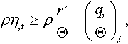
For example, Voigt notation simplifies the customary three-by-three matrix representation of the symmetric second-order stress tensor (refer, for instance, to (2.34)) to a single column matrix with six independent components. Similar reductions are accomplished for matrix representations of the fourth-order elasticity tensor, third-order piezoelectric and piezomagnetic coupling tensors, and second-order strain tensor. With use of this shorthand notation, the constitutive equations (9.90a)–(9.90d), for the special case of a fully coupled TEME material with hexagonal crystal symmetry (i.e., the C6v crystallographic symmetry group), can be presented in matrix form as
where C66 = 1/2(C11 − C12). Clearly, crystal symmetry considerations greatly reduce the number of unknown material constants, which in turn reduces the number of experiments needed to completely characterize a material.
9.8 Linear, reversible, thermo-electro-magneto-mechanical processes
In this section, we discuss the wealth of physical phenomena and material behavior that can be described by the constitutive equations (9.90a)–(9.90d) and characterized as linear, reversible, thermo-electro-magneto-mechanical (TEMM) processes. The multiphysics interaction diagram (see Figure 9.2) describes all combinations of linear TEMM processes. Each of the thermal, electrical, magnetic, and mechanical physical effects are defined by their corresponding extensive and intensive variables, marked at the inner and outer quadrilateral corners of the multiphysics interaction diagram, respectively.
The diagonal edges joining the inner and outer quadrilaterals signify the uncoupled processes, i.e., elasticity, polarization, magnetization, and heat capacity. Coupled processes are described through six subset diagrams, each relating two of the four physical effects. Each of the six subset diagrams, the corresponding coupled processes, and the materials that exhibit these properties are highlighted in Table 9.8; also see Figure 9.3.


The coupled processes therein can be categorized as either (1) a primary process—a coupled process that relates the intensive parameter of one physical effect to the extensive parameter of the second physical effect—or (2) a secondary process—a coupled process that is a superposition of two or more primary processes. In other words, primary processes are direct or one-step processes that describe the coupling between any two physical effects, whereas secondary processes are multistep processes that are a superposition of two or more primary effects.
Owing to the linear nature of the constitutive model under consideration, any coupled TEMM effect can be studied as a superposition of the uncoupled and coupled primary processes highlighted in Table 9.8. For example, a linear thermo-electro-mechanical process can be described as the superposition of a linear thermoelectric (pyroelectric) process and a linear electromechanical (piezoelectric) process.
Depending on the smart material being modeled, appropriate terms can be chosen from equations (9.90a)–(9.90d) to describe its behavior. This will be demonstrated in the next section for the special case of piezoelectric materials.
9.9 Specialization of the small-deformation thermo-electro-magneto-elastic framework to piezoelectric materials
As discussed in Section 9.7, ferroelectric materials inherently exhibit nonlinear hysteretic behavior. However, for small deformations and small electromagnetic fields, approximately linear responses are observed in materials such as barium titanate (BaTiO3), poly(vinylidene fluoride), and lead zirconate titanate. Ferroelectric materials like these that operate in a predominantly linear regime are known as piezoelectric materials.
Piezoelectric materials exhibit spontaneous polarization (at temperatures below the Curie point) in the presence of external electric fields. Below the Curie temperature, these materials exhibit a domain structure that lacks a center of symmetry, i.e., the centers of positive and negative charge are not identical. As a result, each unit cell acts as an electric dipole with a positive end and a negative end. Piezoelectrics change dimension in an electric field because the dipole length can be changed by the field: If a voltage is placed across the material, the dipoles respond to the field and change their dipole length, thereby changing the dimension of the crystal. Alternatively, if the crystal is mechanically stretched or compressed, the length of the dipole is changed, creating a voltage difference if there is no conductive path between the two ends of the dipole.
Since a necessary condition for the occurrence of piezoelectricity is the absence of a center of symmetry, piezoelectric materials are intrinsically anisotropic. Since piezoelectricity couples elasticity and polarization, piezoelectric material properties cannot be discussed without reference to the elasticity constant and the electric susceptibility (or electric permittivity); refer to Table 9.7. In what follows, we specialize the linear thermo-electro-magneto-elastic (TEME) framework developed in Section 9.7 to model piezoelectric material behavior. We make the following assumptions for a piezoelectric material operating well below the Curie temperature:
(1) Piezoelectric materials exhibit strains on the order of 10-100 microstrain. Infinitesimal strain theory can thus be used to describe the kinematics.
(2) Piezoelectric materials are used in transducer applications that operate in the low-frequency regime, typically ranging from 10 to 500 Hz. For this range of frequencies, the dynamic behavior of the electromagnetic fields may be ignored. In other words, the electromagnetic fields may be regarded as quasi-static.
(3) Thermal and magnetic effects may be neglected.
(4) The medium is nonconductive. Thus, when an external voltage is applied to the medium, no charge distribution is formed, i.e., σi = 0, and there is no free current, i.e., ji = 0.
These assumptions allow us to simplify the fundamental laws (9.84a)–(9.84j) to
where ø is the electric potential. Note that (9.91d) is a consequence of Faraday's law: in the absence of time-varying magnetic fields, Faraday's law demands that the electric field is curl free, which, in turn, implies that the electric field is the gradient of a scalar potential.
Similarly, the linear constitutive equations (9.90a)–(9.90d) reduce to
where
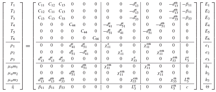
Note that the constitutive equations (9.92a) and (9.92b) relate stress and electric polarization to strain and electric field. Utilizing Voigt notation and imposing hexagonal crystal symmetry (C6v group), we can express (9.92a) and (9.92b) in matrix form as
Exercise
1. Derive a linear reversible framework for the constitutive modeling of magnetostrictive materials, i.e., materials that couple magnetic and mechanical fields. Use the magnetic field h and stress T as the independent variables, and the magnetization m and strain E as the dependent variables. Disregard thermal and electrical effects.