Excel Lesson 1: Getting Started with Excel 2013

In this lesson you will get a general introduction to Microsoft Excel. You will become acquainted with the different areas of Excel, learn how to navigate the workspace, and customize options to create a workspace that suits your needs. You’ll also be briefly introduced to some of the exciting new features of Excel 2013.

What you’ll learn in this lesson:

• • Identifying the different parts of the Excel workspace
• • Using the Ribbon to access commands and features
• • Navigating the Worksheet
• • Exploring the new features of 2013

Starting up

You will work with files from the Excel01lessons folder. Make sure that you have loaded the OfficeLessons folder onto your hard drive from www.digitalclassroombooks.com/Office2013. If you need further instructions, see “Loading lesson files” in the Starting up section of this book.

Getting to know the workspace

In Microsoft Excel, files are called workbooks. In Excel 2013, you can create a new, blank workbook or select from a set of predesigned workbook templates that enable you to quickly get to work. Templates exist for budgets, invoices, lists, reports, and much more. Templates are discussed in greater detail In Lesson 7, “Working with Excel 2013 Templates.”

When you create a new file, a blank workbook containing a single worksheet is displayed. A workbook consists of individual worksheets, each capable of containing its own set of data. By default, each workbook you create contains a single worksheet although a workbook can contain as many as 256 separate worksheets. At the bottom of each worksheet is a tab initially named Sheet1. You can easily rename worksheets by double-clicking the tab and typing the name you wish to use.

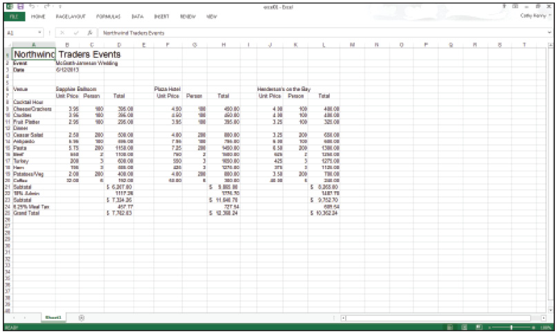
A. Status Bar. B. Row. C. Cell. D. Ribbon Bar. E. Name Box. F. Column. G. Formula Bar.

An Excel worksheet is constructed of columns and rows and is similar in appearance to a grid or bookkeeping ledger. Column headings are arranged along the top of the worksheet window and are labeled alphabetically. Row headings are displayed down the left edge of the worksheet window and are listed numerically.

The basic unit of a worksheet is the cell, formed by the intersection of a row and column. Every cell has a cell address named for that intersection, such as A4 or G11. When you click a cell, the column and row headings appear highlighted, indicating the cell’s address. The cell address also appears in the Name box, located just above column A.

1 Launch Microsoft Excel.

The Backstage displays the files you have recently opened.

2 Choose Open Other Workbooks from the Backstage.

3 Navigate to the Excel01lessons folder and double-click excel01. An Excel document opens to display a worksheet containing three different venue quotes for a fictitious event planning company.

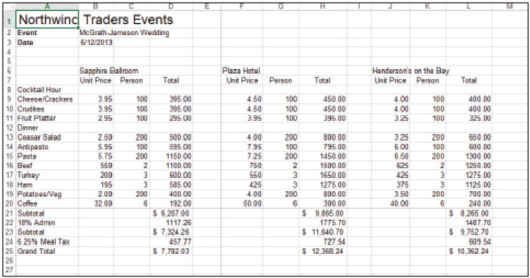
The file named excel01 contains three different pricing quotes for a fictitious events planner.

4 Choose File > Save As and navigate to the Excel01lessons folder. Name the file excel01_work and click Save.

Getting to know the cell pointer

Before we begin exploring the Excel workspace, it helps to get to know the mouse pointer as it takes many different forms in Excel. The pointer appears as the familiar arrow when you are choosing commands. When you move the mouse pointer within the worksheet area the mouse pointer changes its shape to that of a plus sign. As you enter data in a cell, the mouse pointer takes the shape of a cursor.

Since the mouse pointer takes so many different forms depending on the task you are performing it helps to take a moment to review the most basic shapes. The table below describes the mouse pointer shapes in more detail.

Mouse pointer shapes
Shape	Action
	Choose a command
	Select a cell
	Enter or edit data in a cell
	Extend a selection with the AutoFill handle
	Resize columns and rows
	Click to select the current row.
	Click to select the current column.

Using the Ribbon

The Ribbon, which runs along the top of the worksheet window, contains context-sensitive tools and commands to help you organize, calculate, and format your data. It is made up of a series of named tabs, each of which contains a set of related commands. For instance, the Home tab contains a set of frequently-used commands such as Copy and Paste. The names of the tabs are Home, Insert, Page Layout, Formulas, Data, Review, and View. Additional tabs are also displayed when working Charts, Images, and PivotTables.

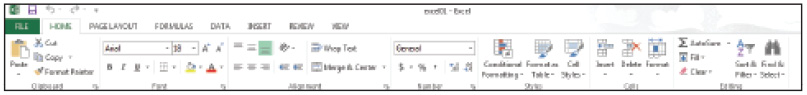
Use the Ribbon to choose commands.

The table below describes the options on the Ribbon in more detail.

Tab	Description
Home	Contains commonly used commands such as format cells, copy and paste, text alignment, and number formats.
Insert	Commands that enable you to insert items into your worksheet including charts, images, text boxes, and SmartArt.
Page Layout	Contains commands that enable you to change the appearance of your printed page. You can set margins, apply themes, change the page orientation, and insert page breaks
Formulas	Contains function library and other commands related to performing calculations.
Data	Contains commands for managing lists of data.
Review	Contains commands such as Spell Checker, Grammar Checker, etc.
View	Commands that enable you to change the display of the worksheet window.

Customizing the Ribbon display

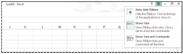
You can collapse the Ribbon, by clicking the Ribbon Display Options button located in the far right corner of the title bar, so that only the named tabs appear across the top of the worksheet window. When you need to choose a command, just click the tab to redisplay the Ribbon and its options. You can also choose to Auto-Hide the Ribbon when you need additional viewing space. When you click the top of the worksheet window the Ribbon is redisplayed.

Collapse the Ribbon to display the named tabs only.

The table below describes the Ribbon Display Options found in the top-right corner of Excel.

Option	Icon	What it Does
Auto-Hide Ribbon		Hides the Ribbon. Click at the top of the Excel window to redisplay it.
Show Tabs		Display tabs only. Click a tab to redisplay the Ribbon.
Show Tabs and Commands		Displays both the Tabs and Commands at all times.

Collapsing the Ribbon

1 Click the Ribbon Display Options button.

The Ribbon Display Options button allows you to alter the Ribbon’s appearance.

2 Choose Show Tabs and then select cell A1.

3 Click the Home tab to redisplay the Ribbon and choose Bold in the Font group.

The Show Tabs command shows the tabs but doesn’t display the Ribbon unless a specific tab is selected. Once a command is selected on the Ribbon or you click elsewhere on the worksheet, the Ribbon disappears.

Hiding the Ribbon

1 Click the Ribbon Display Options button.

2 Choose Auto-Hide Ribbon.

3 Click the top of the Excel window to redisplay the Ribbon.

The Auto-Hide Ribbon command hides the Ribbon from view. When you click the top of the worksheet window, the Ribbon is redisplayed.

Once you choose a command or click elsewhere on the worksheet, the Ribbon disappears.

To quickly collapse the Ribbon, right-click anywhere within the Ribbon and choose Collapse the Ribbon.

Exploring the Status bar

The Status bar appears at the bottom of the worksheet window and provides updates on the current worksheet. Messages appear in the lower left corner to tell you what a command does, or what you should do next, to execute a command. For instance, when entering data in a cell the Status bar displays ENTER in the lower left corner.

The Status bar displays the word ENTER when entering data in a cell.

The Status bar also contains a set of buttons that enable you to change the view of your worksheet. You can switch between Normal, Page Layout, and Page Break Preview modes. Using the Zoom slider, you can enlarge or reduce the size of the worksheet display.

Switching display modes

The default viewing mode in Excel is the Normal mode, and it is primarily used when you are working with your data. There are times when you want to switch the display to see what your worksheet will look like when printed, or you may just want to view where the page breaks will occur, and you can use various display modes to see these things. You can quickly change the viewing mode of your worksheet by using the buttons in the Status bar. You’ll learn more about printing in Lesson 2, “Creating a Worksheet in Excel 2013.”

1 Switch to Page Layout mode by clicking the Page Layout button.

Choose the Page Layout mode.

2 Switch to Page Break Preview mode by clicking the Page Break Preview Button.

3 Click Normal to return the regular viewing mode.

Change the size of the worksheet display

You may need to change the size of your worksheet display, especially if you are working with data that extends beyond the visible area. Using the Zoom tool in the Status bar, you can quickly reduce or enlarge the worksheet display.

Change the size of your worksheet display by dragging the Zoom slider.

1 Click and drag the Zoom slide to enlarge the display area to 125%.

2 Drag the slider to 100% to return the view to its original size.

Using the Quick Access Toolbar

The Quick Access Toolbar is displayed at the top left of the Excel window and provides single-click access to frequently-used commands such as Save and Undo. You can customize the toolbar to add additional commands that you use frequently.

1 Click the Customize Quick Access Toolbar button.

Add your favorite commands to the Quick Access Toolbar to gain single-click access.

2 Click New to add the New command to the toolbar.

3 Click the Customize Quick Access Toolbar again and click Open to add the Open command to the toolbar.

Using the Formula bar

The Formula bar appears just below the Ribbon and displays the contents of the active cell. When you type data in a cell, the Formula bar activates and displays the data as you type.

1 Click in cell A6 and type Venue.

As you type, the data appears in the Formula bar.

Notice also the appearance of three buttons to the left of the Formula bar. These buttons enable you to confirm or cancel what you are entering or a Function within the cell. Formulas will be discussed in greater detail In Lesson 4, “Using Formulas in Excel 2013.”

The buttons in the Formula bar
Button	Action
	Confirms the current entry. Equivalent to pressing Enter.
	Cancels the current entry. Equivalent to pressing Esc.
	Opens the Insert Function dialog box.

To use the Formula bar after data has been entered:

1 Activate the cell by clicking it.

2 Move the mouse pointer to the Formula bar area.

3 When the cursor appears, click within the Formula bar to set the insertion point.

Moving around the worksheet

The active cell in a worksheet always appears with a dark outlined border. To activate another cell using the mouse, move the mouse pointer to the cell you wish to use and click it. For example, you can click cell F13 to make it active.

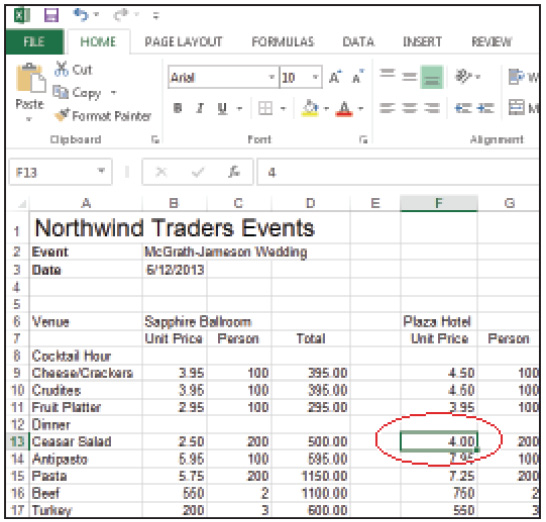
The active cell in a worksheet appears with an outlined border.

You can also move the cell pointer around the worksheet by using the keyboard. The table below discusses the keys for navigating the worksheet with the keyboard.

Navigating the worksheet with the keyboard
Key	Movement
Up, Down, Left, Right	Moves one cell to the left, right, up or down
Ctrl Up, Down, Left, Right	Moves to the next cell of data separated by a blank cell
Tab	Moves one cell to the right
Shift Tab	Moves one cell to the left
Home	Moves to the first cell in the row
Ctrl + Home	Moves to cell A1
End + Left	Moves to the next non-blank cell to the left
End + Right	Moves to the next non-blank cell to the right
End + Up	Moves to the next non-blank cell above.
End + Down	Moves to the next non-blank cell below.
Ctrl + End	Moves to the last cell containing data
PgUp	Moves up one screen
PgDn	Moves down one screen
Ctrl + PgUp	Moves to the next worksheet
Ctrl + PgDn	Moves to the previous worksheet

Moving to a specific cell

You can quickly move to a specific cell within a worksheet by typing the cell address in the Name box that appears to the left of the Formula bar.

1 Click the Name box.

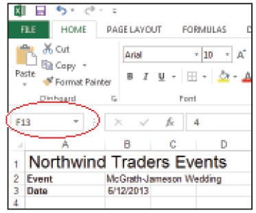
To quickly move to a specific cell, type the cell address in the Name box.

2 Type D11 and press Enter or Return on your keyboard to move to cell D11.

Using the scroll bars

The scroll bars, located along the right edge and bottom of your worksheet window, offer the quickest way to navigate a worksheet with the mouse or touch screen. Each scroll bar consists of a scroll box, scroll arrows, and the scroll bar. The scroll box, located within the scroll bar, changes size depending on where you are in the worksheet. When you are at cell A1, the scroll box fills the entire scroll bar. As you drag the bar further away from A1, the scroll box decreases in size.

A. Scroll Arrow. B. Scroll Box. C. Scroll Bar.

Exploring what’s new in Excel 2013

Microsoft has been busy adding new features designed to help you display your data visually, and has provided you with a new streamlined interface. Let’s take a quick look at some of the new features Excel 2013 has to offer.

Templates help you get started right away

Excel’s Backstage view, which appears whenever you launch Excel or choose File > New, displays a set of professionally designed worksheet templates. When you create a worksheet from a template, you need only plug in your data and the worksheet will update automatically.

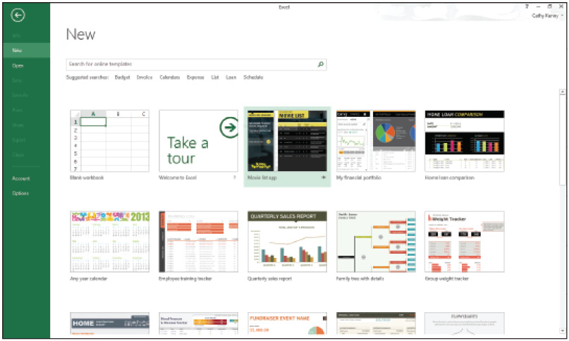
Excel’s Templates take the design-work out of your hands and let you get started immediately.

Excel offers thousands of template choices to help you get up and running. From Invoices and Budgets, to Sales Reports and Cash Flow Statements, Excel has templates for virtually every type of business or organizational need. There are also a wide assortment of personal templates, such as a Home Construction Budget, a Group Weight Loss Tracker, and the ability to keep track of your movie collection with the Movies List. Excel also makes it easy to search through thousands of online templates with its built in Search box. For more information on using Excel’s templates, see Lesson 7, “Working with Excel 2013 Templates.”

Quick analysis gets down to business

With the new Quick Analysis button, you can instantly produce visual snapshots of your data. After selecting a range of data, click the Quick Analysis Button and choose from the selected options. Add special Formatting, create a quick Chart, add a line of Totals, produce a PivotTable, or add Sparklines. For more information on the Quick Analysis Tools, see Lesson 8, “Advanced Data Analysis in Excel 2013.”

Get a quick visual of your data with the new Quick Analysis tools.

Flash Fill reduces data entry drudgery

One of the more tedious aspects of working with a program like Excel is that before you can analyze your data, you first have to enter it into your worksheet. Excel 2013 introduces Flash Fill, which aims to reduce the drudgery that is data entry. As you enter data, Excel analyzes the data for any patterns that may exist and if it detects any, fills the rest of the Information for you. For more information on using Flash Fill, see Lesson 6, “Working with Data.”

Excel aims to reduce data entry time by anticipating patterns and filling the remainder in for you.

Chart recommendations remove the guesswork

Not sure which chart type is the best fit for your data and the message you want to convey? With Excel’s new Chart recommendations, you needn’t ever second guess yourself again. Just select the data you want to chart and choose Recommended Chart’s, from the Insert tab. Excel will recommend a set of charts based on your data. For more Information on charts, see Lesson 5, “Working with Charts.”

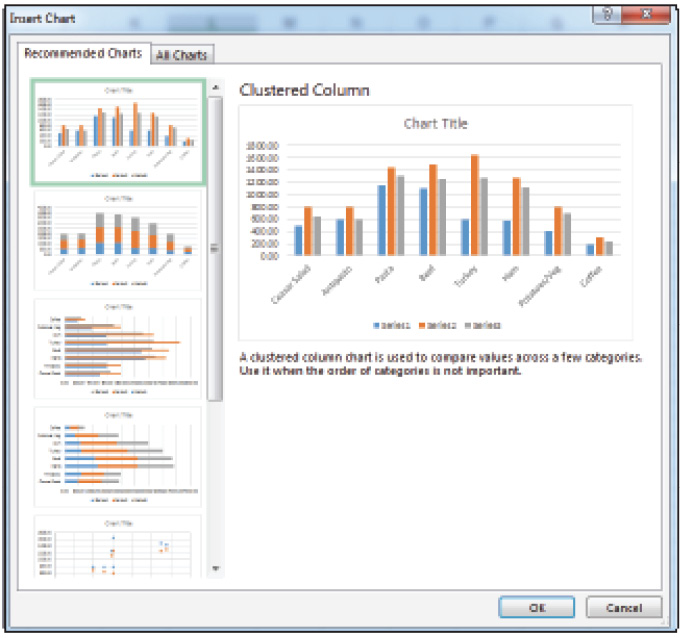
Use Chart Recommendations when you are not sure which chart type best suits your data.

Filter your data with slicers

You can use slicers to filter your data using more than one value. The slicer is built-in to the Table feature and an icon is displayed to let you know when your data has been filtered. To learn more about Data Slicers, see Lesson 8, “Advanced Data Analysis in Excel 2013.” While the slicer functionality first appeared in Office 2010, it has been streamlined significantly for Office 2013.

Filter your data on multiple values using the new Data Slicers.

You’ve now completed this lesson. Now that you are familiar with the workspace in Excel, you are ready to begin creating new worksheets and working with your data.

Self study

1 In the excel01_work document, use the keyboard to navigate the worksheet. Press Ctrl+End to move to the last active cell in the worksheet. Press Ctrl+Home to move to cell A1.

2 Double-click cell A3 and edit the text to read Date of Event.

3 Add the Print Preview and Print command to the Quick Access Toolbar.

Review

Questions

1 What is the difference between a worksheet and a workbook?

2 Name at least two different ways the cell pointer is displayed.

3 What is the quickest way to move to a specific cell in your worksheet?

4 How do you change the size of the display of your worksheet?

5 How you do collapse the Ribbon?

Answers

1 The difference between a worksheet and a workbook is that a workbook is a collection of separate worksheets stored together in a single file, whereas a worksheet is single sheet on which you store information.

2 The cell pointer appears as an arrow when selecting commands from menus and toolbars, a plus sign when within the worksheet, and a cursor while you are entering data.

3 For the quickest way to move to a specific cell in your worksheet, enter the cell’s address in the Name box.

4 To change the display size of your worksheet, click and drag the Zoom slider tool in the Status bar.

5 To collapse the Ribbon, click the Ribbon Display Options button and choose Show Tabs or right-click anywhere within the Ribbon and choose Collapse Ribbon.