Excel Lesson 3: Formatting a Worksheet

In this lesson, you will learn how to format a worksheet in Excel. You will change the format of numeric entries, apply fonts, change font sizes, align text within cells, and across multiple columns. You’ll learn how to use the Format Painter and Cell Styles to apply styles to multiple ranges. Finally, you’ll learn how to use color-coordinated themes in your worksheets.

What you’ll learn in this lesson:

• • Formatting numeric entries
• • Changing the font and font size
• • Adding borders and shading
• • Applying conditional formatting
• • Changing row and column sizes

Starting up

You will work with files from the Excel03lessons folder. Make sure that you have loaded the OfficeLessons folder onto your hard drive from www.digitalclassroombooks.com/Office2013. If you need further instructions, see “Loading lesson files” in the Starting up section of this book.

Understanding cell formats

Before we talk about cell formatting, you must understand how Excel treats data. Excel categorizes data into three different types: numbers, text, and dates or times. Numbers, or values, consist of numeric data that will be used in calculations or formulas. There are also numbers on which you would never perform calculations, such as zip codes, social security numbers, product codes, or phone numbers.

Text also appears to be a straightforward concept. Text includes alphanumeric data that can be used in headings and other descriptive labels, for example, Sales 2001 or Northwest Region. When you enter a date, you might also think of it as a text-based entry, for example, March 27, 2013 or even 3/27/2013. Dates, in all actuality, are converted to a date value when entered, since you can perform calculations with dates.

When numbers are entered in a worksheet cell, Excel automatically applies a General format, unless it recognizes the value in some other way. For instance, if you enter a dollar ($) sign with the value, Excel assigns the Currency format. If you enter a percent (%) sign, it applies a percentage format. If you enter a value with a decimal point, Excel assigns the Number format.

When you enter numbers such as zip codes and social security numbers in a cell, Excel thinks they are values and treats them as such. In the case of zip codes, Excel automatically removes any leading zeroes from the number, (for example, 02124 becomes 2124), and converts it to a number. In these cases, you must intervene and let Excel know that the data you are entering is actually a text entry.

The following table explains the different types of cell formats that Excel uses.

Cell formats
Format	Description
General	Applies no specific format. Will display decimal point if initially entered.
Number	Displays decimal point and two decimal places.
Currency	Displays the currency symbol to the immediate left of the value and a minus sign in front of negative numbers.
Accounting	Displays the currency symbol to the left edge of the cell, lines up decimal points, and encloses negative values in parentheses.
Short Date	Displays the date in mm/dd/yyyy format: 3/24/2013
Long Date	Displays date in expanded format: Monday, March 25, 2013
Time	Displays time in hh:mm:ss format: 12:19:20 PM
Percentage	Displays the percent symbol and rounds up
Fraction	Displays the value as a fraction
Scientific	Displays the value using scientific notation
Text	Data entered will be treated as text and will not be used in calculations.

Changing number formats

You can format your numeric entries using a variety of predefined formats. You can also create and apply custom numeric formats for values such as phone numbers and zip codes.

In this first lesson, we will format a range of values using a variety of number formats.

Applying a numeric format

The next steps show an example of how to use this feature.

1 Launch Excel and open the file named excel03 from the Excel03lessons folder.

2 Select range B9:B20.

3 In the Number section of the Home tab, click the arrow to display the Format drop-down menu.

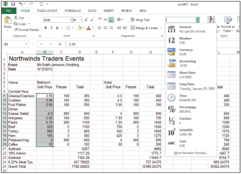
First select the range of cells and then assign a format to your values.

4 Choose Number.

Excel adds a decimal point and two digits (two decimal places) after each value in the range.

Commonly-used numeric formats
Icon	Name	Action
	Accounting (Currency)	Adds the currency symbol and two decimal places
	Percent	Adds the percent sign and zero decimal places
	Comma	Adds the thousands separator and two decimal places
	Increase Decimal	Increases the decimal place setting by 1
	Decrease Decimal	Decreases the decimal place setting by 1

Changing the number of decimal places

By default, Excel rounds values with the Number format to two decimal places. You can increase or decrease the decimal place value accordingly. The following steps show an example of how to use this feature.

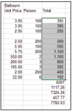
1 Select range D24:D25. Notice that all numbers in this range have four decimal places.

2 In the Number section of the Home tab, click the Decrease Decimal button () three times.

3 Excel rounds down the value and displays the result with two decimal places instead of the original four. The value in cell D25 now reads 7782.03.

4 Perform steps 1–3 for ranges H24:H25 and range L24:L25.

Adding the thousands separator

Excel automatically adds the thousands separator when the Currency or Accounting format is applied. The Comma Style format can be used when you want the thousands separator but not a currency symbol. Follow the next steps for an example of how to use this feature.

1 Select range D9:D20.

2 Press and hold the Ctrl key and select ranges H9:H20 and L9:L20.

3 In the Number section of the Home tab, click the Comma Style button. Excel adds the thousands separator to the values and adds two decimal places.

4 Click the Decrease Decimal button on the Home tab twice to remove the decimal place setting.

Click the Decrease Decimal button to remove the two decimal spaces.

Assigning the currency format

The next steps show an example of how to assign the currency format.

1 Select range D21:D25.

2 Press and hold the Ctrl key and select ranges H21:H25 and L21:L25.

3 From the Home tab, choose Number Format.

4 From the Number Format list, choose Currency to apply this style to the selected cells.

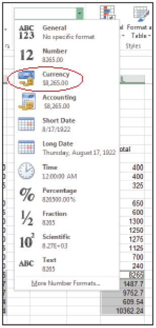
Assign the Currency format to a range of cells.

Assigning the accounting format

The next steps show an example of how to assign the accounting format.

1 Select range D21:D25.

2 Press and hold the Ctrl key and select ranges H21:H25 and L21:L25.

3 From the Home tab, choose Number Format.

4 From the Number Format list, choose Accounting. Notice how the Accounting format looks slightly different than the Currency format but the dollar signs, commas and decimals remain.

Values assigned the Accounting format look slightly different than the Currency format.

Assigning the text format

The next steps show an example of how to format the text.

1 Type the label Contact Number in cell A4.

2 Click in cell B4.

3 From the Home tab, choose Number Format.

4 From the Number Format list, choose Text.

5 Type (800) 555-1212 in cell B4 and press Enter.

Creating custom formats

When formatting data, you can choose from among the built-in formats or you can assign a custom format for specialized data. Follow the next set of steps for an example of how to create custom formats.

1 Click in cell B4.

2 From the Editing group on the Home tab, choose Clear.

3 From the Clear list, choose Clear All.

4 Type 8005551212 in cell B4 and press the Enter key.

5 Click back on cell B4 and from the Home tab, choose Number Format.

6 In the drop-down menu choose More Number Formats.

Use Special Formats for items such as zip codes and phone numbers.

7 In the Format Cells dialog box, select Special as the Category.

8 From the Type section, select Phone Number.

9 Click OK to apply the format.

Changing the font and font size

In addition to changing the display of numeric data, you can add visual interest to your worksheets. Some of the changes you can make include font and font size, the color of the text, the background color of the cell, and text attributes such as bold, italic, and underline.

Changing the font

The following set of steps show an example of how to change the font.

1 Select range A1:L27.

2 From the Home tab, choose Font from the Font group.

3 Select Calibri from the list. Notice that your selected worksheet cells display a preview of the font as you move over a font name in the list.

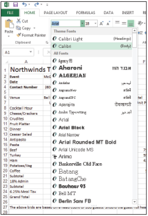
Change the manner in which your data is displayed with the Font option.

Changing the font size

The following set of steps show an example of how to change the size of the font.

1 Select range A2:L27.

2 From the Home tab, choose Font Size to display the drop-down list of font sizes.

3 Select 12.

Click the Increase Font Size or Decrease Font Size buttons to quickly adjust the size accordingly.

Changing the color of your text

The following set of steps show an example of how to change the color of text.

1 Select range A1:B4.

2 From the Home tab, click the arrow to the right of the Font Color button to display the color palette.

3 Select Blue. Notice that the Font Color icon now reflects the change in color. You can apply the same color to another range of cells by clicking the icon because Excel saves the color that was last used.

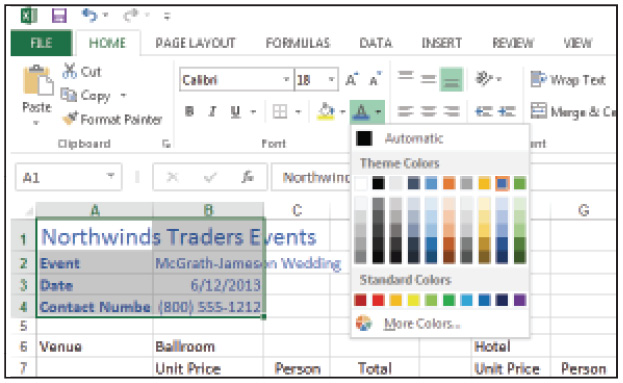
For on-screen displays, make use of color.

Changing the background color of cells

The following set of steps show an example of how to change the background color of cells.

1 Click cell D25.

2 From the Home tab, click the arrow to the right of the Fill Color button to display the color palette.

3 From Standard Colors, select Orange. Notice that the Fill Color icon now displays the paint color you selected.

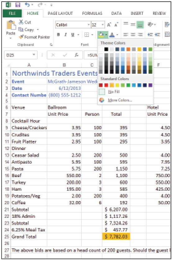
Change the background color of cells to draw attention to important data.

Changing text attributes

Another way to add visual interest to your worksheets is to use text attributes, which works regardless of the font you have chosen. Your choices are bold, italics, underline, and double-underline. The next set of steps show an example of how this feature works.

1 Select range B7:D7.

2 Press and hold the Ctrl key and select ranges F7:H7 and J7:L7.

3 From the Home tab, choose Bold.

4 Select ranges A9:A11 and A13:A20.

5 From the Home tab, choose Italic.

Text attributes can help set headings apart from the rest of the worksheet data.

Modifying row heights and column widths

By default, column widths and row heights are set to predefined measurements. If the data in a worksheet is larger than the column width or row height allows, Excel will alert you depending on the data type. If text is longer than the column width, Excel truncates the text if the cell to the immediate right contains data. Otherwise, the text continues to be displayed. If a numeric entry is longer than the current column width, Excel displays a series of number signs (########) in the cell. Row heights are set to adjust automatically when you change the size of your data.

Change the column width

The next set of steps show an example of how to change the width of columns.

1 Click in cell L25.

2 From the Cells group on the Home tab, choose Format.

3 Select Column Width from the resulting menu to display the Column Width dialog box.

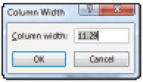
Change the width of a column by typing an amount in the Column Width dialog box.

4 Type 12 In the Column Width text box, and then click OK.

Changing the column width with the mouse

The next set of steps show an example of how to change the width of columns with the mouse.

1 Click the border separating columns A and B.

2 Click and drag the mouse to the right.

3 Release when column A displays the label Contact Number in its entirety.

Change the width of a column by clicking and dragging the column border.

Changing the column width automatically

You can quickly adjust the column width to accommodate the longest entry.

1 Select any column from the worksheet.

2 From the Cells group on the Home tab, choose Format.

3 Select AutoFit Column Width to set that column to auto-fit the width depending on the contents.

You can also double-click the border between the column headings to adjust the column width to the widest entry.

Changing the row height

The next set of steps show an example of how to adjust the height of a row.

1 Click the border separating rows 5 and 6.

2 Click and drag the mouse down.

3 Release when the row is the height you desire.

Excel automatically adjusts the height of a row when you change the size of the data within the row.

Changing the row height automatically

You can quickly adjust the row height to accommodate the tallest entry.

1 Select row 5 from the worksheet.

2 Choose Format from the Cells group of the Home tab.

3 Select AutoFit Row Height.

Double-click the border between the row headings to automatically adjust the height of a row.

Cell alignment

By default, Excel automatically aligns numeric data to the right edge of a cell and text entries to the left. For the most part, numeric entries generally stay aligned to the right for consistency’s sake. There are many different options for aligning text within a worksheet. Text can be aligned within a cell or across a range of cells. You can change the horizontal and vertical placement of text within a cell and you can also wrap extra-long text entries within a single cell.

Excel automatically aligns text to the left edge of the cell and numbers to the right.

Aligning text within cells

You can change the alignment of text both within the columns and rows. That is, between the column widths and the row heights. When you increase the width of a row, data can be aligned between the top and bottom edges of the cell.

1 Select range B7:D7.

2 Press and hold the Ctrl key and select ranges F7:H7 and J7:L7.

3 On the Home tab in the Alignment group, click the Center button. Excel centers the headings within the selected cells.

Merging and centering columns

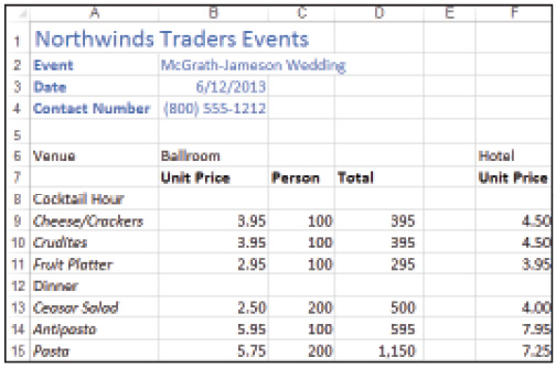
You can center a heading over multiple columns with the Merge and Center command. When you merge a range of cells, all the cells are converted to a larger single cell. For instance, in our example we want the heading for the venue type to be centered over the column headings Unit Price, Person, and Total.

1 Select range B6:D6, which contains both the heading we want to center and the columns to center it over.

2 From the Home tab, choose the Merge & Center command from the Alignment group.

3 Excel merges cells B6, C6, and D6 and centers the heading Ballroom over all three columns.

4 Merge and Center range F6:H6 and J6:L6.

When a heading spans multiple columns, use the Merge & Center command to center the heading over all the columns.

Wrapping text

Excel has a number of sophisticated text handling tools that you would normally only find in a word processing program such as Microsoft Word. As Excel has grown more powerful and easier to use, it has added the ability to manipulate text within worksheet cells. For example, the Wrap Text command allows you to wrap extra-long text within a single cell.

The following set of steps shows an example of how to wrap text.

1 Click cell A27.

2 Choose Wrap Text from the Alignment group on the Home tab.

Excel enlarges the height of row 27 and wraps the extra-long notation within cell A27.

Rotating text

Another advanced text editing tool is the ability to rotate text within a cell. This can be useful when a heading is much longer than the data it is describing, or when you’d like to fit more data on a single page.

Follow the next set of steps for an example of how to rotate text.

1 Select range B7:D7.

2 Choose Orientation from the Alignment group on the Home tab.

3 Select Angle Counterclockwise.

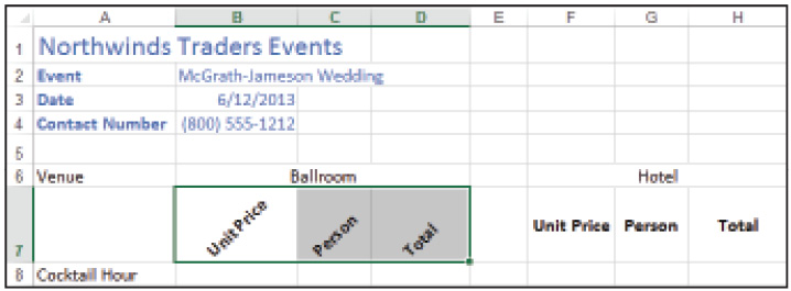
Text alignment helps when you need to make more room on a page.

When you apply formatting to a cell, the format is either On or Off. A format that is applied to the current cell will appear highlighted to indicate that it is on.

4 Click the Orientation button again and choose Angle Counterclockwise again to turn off the format from range B7:D7.

Borders and shading

Just as text and number formats can help guide the eye in a worksheet, so too can the use of borders. A border can be applied to all four sides of a cell in a variety of line styles.

There are two ways to add a Border: you can add a predesigned border to a selected range of cells or you can draw your own, changing the line style and color yourself.

Applying a border

The following steps show an example of how to add a border.

1 Select range B6:D7.

2 Choose Borders from the Font group on the Home tab.

3 Select Outside Borders.

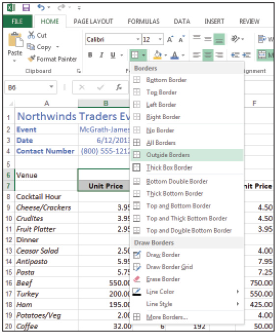
Add borders to your worksheet to help draw the eye.

4 Click another cell so you can view the thin border.

Once you select a Border style, the Border icon maintains that style until you pick a new one. Select each range of cells and click the Border icon to apply the style.

Drawing a border

Excel automatically uses a single black line style when you draw a border. You can change both the line style and color of a border you drawn, as illustrated by the next set of steps.

1 From the Font group choose Borders.

2 Choose Line Style and select the Thick-Dashed line style. The cell pointer changes its shape into that of a pencil.

3 Choose Borders again, click Line Color and select Green.

4 Click and drag the pencil around range F6:H7 to add the border.

5 Press the Esc key on the keyboard when you have finished to remove the pencil cell pointer.

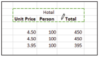
Draw a custom border around a range of cells.

Erasing a border

Just as there are two ways to add a border, there are two ways to remove a border. When you apply a border, you select the range of cells and then pick the border you want to use. To remove a border, select the range of cells and choose No Border from the Border command. You can also use the Erase Border command to erase the border by clicking each cell that has a border.

Here is an example of erasing a border using the No Border option:

1 Select range B6:D7.

2 From the Home tab, choose Border.

3 Choose No Border from the displayed list.

The following is an example of erasing a border with the Border Eraser:

1 From the Home tab, choose Border.

2 Choose Erase Border. The mouse pointer is displayed as an eraser.

3 Click the eraser on the edge of each cell in range F6:H7 to remove the border.

Remove a border from a range of cells with the Eraser.

4 Press the Esc key when finished to return the pointer back to normal.

Copying cell formats

Excel’s Format Painter tool is essential when formatting a worksheet. With this tool, you can quickly and easily copy a format from one cell to another with a single click. Follow the next set of steps for an example.

1 Select cell D25.

2 In the Clipboard group, choose the Format Painter. The mouse pointer now includes a paint brush.

Copy formats from one cell to another with the Format Painter command.

3 Click cell H25 to apply the formatting.

4 Repeat step 2 and 3 to copy the format to cell L25.

To apply formatting to multiple cells, double-click the Format Painter and click each cell to apply. Press Esc when you are done.

Working with cell styles

A style is a collection of formatting stored under a single name. A style can consist of alignment, numeric formats, borders, fonts, shading, and a host of other attributes. To apply that collection of attributes, you need to assign the style rather than each attribute individually.

Excel comes with a number of predefined styles from which to choose; you can also create your own.

Applying cell styles

Follow the next set of steps for an example of how to apply styles to cells.

1 Select range A8:A11.

2 From the Styles group choose Cell Styles.

Assign cell styles to maximize visibility.

3 Select 40% - Accent 2.

4 Select range A12:A20.

5 From the Home tab, choose Cell Styles.

6 Select 40% - Accent 1.

7 Click cell A8, press and hold the Ctrl key, and click cell A12.

8 From the Home tab, choose Cell Styles.

9 Select Heading 3.

10 Hold the Ctrl key and click cells A21, A23, and A25.

11 From the Home tab, choose Cell Styles.

12 Select Total.

Clearing a style

You can easily remove the formatting from a cell without removing its contents with the Clear command, as the following set of steps illustrates.

1 Select range A9:A11.

2 From the Editing group, choose Clear.

3 Select Clear Formats from the resulting menu to remove the themed cell style.

Creating a style

If you don’t want to use any of Excel’s built-in styles, you can create your own styles and save them for future use. Once you create a style, it appears at the top of the Styles menu under the Custom category. The easiest way to create a style is to assign the appropriate formats to the cell first, as demonstrated by the following steps.

1 Click cell B6.

2 Change the Font to Bauhaus 93, the size to 14, the color to Blue, and add a Border to the Bottom of the cell.

3 From the Styles group, choose Cell Styles, and then click New Cell Style.

4 Type Heading Column in the Style name text box and click OK.

You can create your own custom styles and save them for future use.

Modifying a style

Another way to create a custom style is to take an existing style, change an attribute or two, and save it as a new style.

1 From the Styles group, choose Cell Styles to display the Style Gallery.

2 Right-click the Heading Column style at the top of the Style Gallery that you just created and choose Modify.

Rather than start from scratch, modify an existing style to suit your needs.

3 Click Format in the resulting dialog box, and then click the Font tab.

4 Change the size to 12.

5 Click OK twice to save the modifications.

Merging styles from other worksheets

When you create a style, Excel stores the style in the worksheet in which it was created. You can use custom styles with other worksheets, but you must first merge them in to the current worksheet.

1 Open a new worksheet using the File > New command. Choose Blank workbook.

2 Choose Cell Styles from the Styles group.

3 Select Merge Styles.

4 Select excel03 to copy the styles into the new, blank workbook.

You can merge cell styles from other workbooks into the current file.

5 Click OK.

6 In the resulting dialog box, click No to keep the styles in the current workbook intact and merge the custom styles only.

7 Choose File > Close. We won’t be working with this file so you don’t need to save it.

Using conditional formatting

Excel’s conditional formatting options let you draw attention to important points in your data set based on a certain set of criteria. You could, for instance, highlight values that are greater than a certain value; highlight sales data that falls within the top 10%; or highlight testing values that are above average. By using color, symbols, and other special attributes, you can show data at a glance that might be on the rise or falling below expectations.

Conditional formatting is based on a set of predefined rules. For instance, the rule that states Format All Cells Based on Their Values formats cells using a graduated color scale based on a set of defined values. There are five different categories of rules and a number of options within each category that you can use.

Conditional formatting rules
Icon	Highlight Cell Rules	Description
	Highlight Cells Rules	Highlights cells based on a defined value.
	Top/Bottom Rules	Highlights values based on a defined ranking.
	Data Bars	Adds a data bar to the cell to represent the value; the longer the bar, the larger the value.
	Color Scales	Applies a gradient color scale to a value and the color indicates where the value falls within a range.
	Icon Sets	Adds a set of icons to represent the values in a range of cells.

To demonstrate conditional formatting, we will open a new worksheet from the Excel03lessons folder. But first, save and close the current event planning worksheet we have been using.

1 Go back to the excel03 worksheet and choose File > Save As.

2 In the Office Background, click Computer and navigate to the Excel03lessons folder.

3 In the file name text box, type _formats at the end of the current file name.

4 Click Save, and then choose File > Close.

Using conditional formatting

Follow the next set of steps for an example of how to use this feature.

1 Choose File > Open.

2 Navigate to the Excel03lessons folder and double-click the file named excel03_grades.

3 Select range A4:E37.

4 From the Style group, choose Conditional Formatting.

5 Select Top/Bottom Rules and select Top 10%.

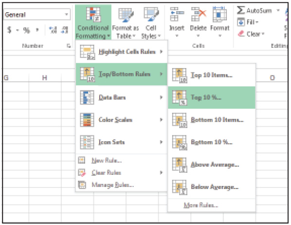
Instantly highlight important data with Conditional Formatting.

6 Click OK. Excel highlights the grades that fall within the Top 10%.

Removing conditional formatting

You can remove conditional formatting from an entire worksheet or a specified range, as the follow example indicates.

1 Select range A4:E37.

2 Choose Conditional Formatting again.

3 Choose Clear Rules.

4 Select Clear Rules from Selected Cells.

Creating a new rule

If the predefined rules are not what you are looking for, you can create your own, including specifying the formatting you want to apply should the conditions be met. The next set of step shows you an example of how to use this feature.

1 Select range E4:E37.

2 From the Style group choose Conditional Formatting again.

3 Choose New Rule.

4 From the Rule list, select Format only cells that contain.

5 In the Format only cells with sections, select Greater Than from the drop-down menu adjacent to the Cell Value field.

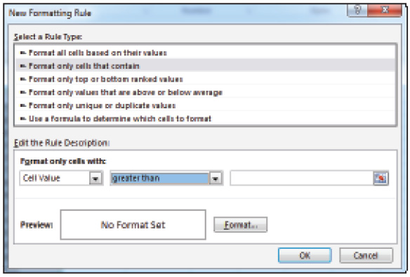
Create a New Rule to make your data standout when it meets specific criteria.

6 Type 2000 in the box adjacent to Greater Than.

7 Click Format and choose the Fill tab.

8 Select the color Blue.

9 Click OK twice. Excel highlights all scores that are higher than 2000.

Using page themes

Page themes are a collection of color-coordinated color schemes and font families for use in a single worksheet. Each theme contains a set of predefined colors, fonts, and attributes that have been professionally designed and coordinated. You can also swap out different parts of each theme to suit your individual needs. You can, for instance, pick a new font set to use or select a different color scheme. You can also adjust the settings for objects added to your worksheets with the Drawing tools.

Applying a theme

Follow the next set of steps for an example of how to apply a theme.

1 From the Page Layout tab, choose Themes from the Themes group.

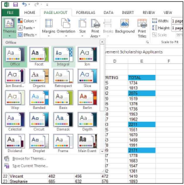
Use Page Themes to design color-coordinated worksheets.

2 Select Integral from the theme list.

Excel changes the appearance of your worksheet, including any cells that make existing use of Cell Styles or colors.

Changing the color scheme

Follow the next set of steps for an example of how to change the color scheme of your worksheet.

1 From the Page Layout tab in the Themes group, choose Colors.

2 Select Blue Green.

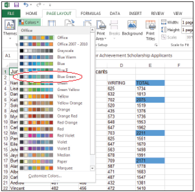
Swap out one color set for another in the Page Theme.

Changing the font set

Follow the next set of steps for an example of how to change the font set used by your worksheet.

1 From the Page Layout tab, choose Fonts.

2 Select Corbel.

Pick a new Font family to use in the Page Theme.

Changing the effects

Follow the next set of steps for an example of how to change the effects used in your worksheet.

1 From the Page Layout tab in the Themes group, choose Effects.

Select the effects to add to drawn objects in a worksheet.

2 Select Glow Edge.

3 Choose File > Save As, and navigate to the Excel03lessons folder. Type excel03_grades_format as the file name, and click Save.

Self study

Perform the following exercises in the excel_formats file.

1 Use the Format Painter to copy the formatting from cell B6 to cells F6 and J6.

2 Add a Top and Bottom Double Border to ranges B21:L21, B23:L23, and B25:L25.

3 Change the Fill Color for cells D25 and H25 to No Fill.

Review

Questions

1 What is the difference between the Currency and Accounting cell formats?

2 How do you add the thousands separator to a value without also adding the currency symbol?

3 What is the quickest way to center a heading over multiple columns?

4 How do you resize a column?

5 What is a Cell Style?

Answers

1 Both the Currency and Accounting formats add the currency symbol and decimal places to a value. But the Currency format displays the currency symbol to the immediate left of the value and displays negative numbers with the negative symbol (-). The Accounting format displays the currency symbol at the far left of the column and displays negative numbers using parentheses.

2 To add the thousands separator to a value without also adding the currency symbol, select the cell containing the value you want to format. Choose Comma Style from the Home tab. Excel adds the thousands separator and two decimal places to the value.

3 The quickest way to center a heading over multiple columns is to start by selecting the range of cells containing the heading and the columns you want to center. Then choose the Merge & Center command from the Home tab.

4 You can quickly resize a column by clicking and dragging the column border to the right. Double-click the border to automatically resize the column to its longest entry.

5 A Cell Style is a collection of formatting attributes saved under a single name. You can apply a cell style to a cell or range of cells by first selecting the data, and then choosing the name from the Cell Styles menu in the Home tab.