Excel Lesson 6: Working with Data

In this lesson, you will learn how to manage lists of information in Excel. You’ll begin by learning the proper way to arrange a list. Then you will learn how to sort records, apply filters to view selected records, and search a list. You will also learn how to remove duplicate entries from a list and how to extract records.

What you’ll learn in this lesson:

• • Entering data in a list
• • Sorting data
• • Using filters
• • Removing duplicates
• • Extracting data

Starting up

You will work with files from the Excel06lessons folder. Make sure you have loaded the OfficeLessons folder onto your hard drive from www.digitalclassroombooks.com/Office2013. If you need further instructions, see “Loading lesson files” in the Starting up section of this book.

Working with lists

With Excel, you can easily manage data in a list. After information is organized into a list format, you can find and extract data that meets certain criteria. You can also sort information in a list to put into a specific order, and you can extract, summarize, and compare data.

Database terms

A list, also known as a database, is information that contains similar sets of data, such as a phone directory. Information in a list is organized by categories or fields. Each column in a list contains a heading or field name that determines the type of information entered in that column. You enter data in a row to form a record. Once information is organized in a list, you can filter, sort, extract, and summarize the data.

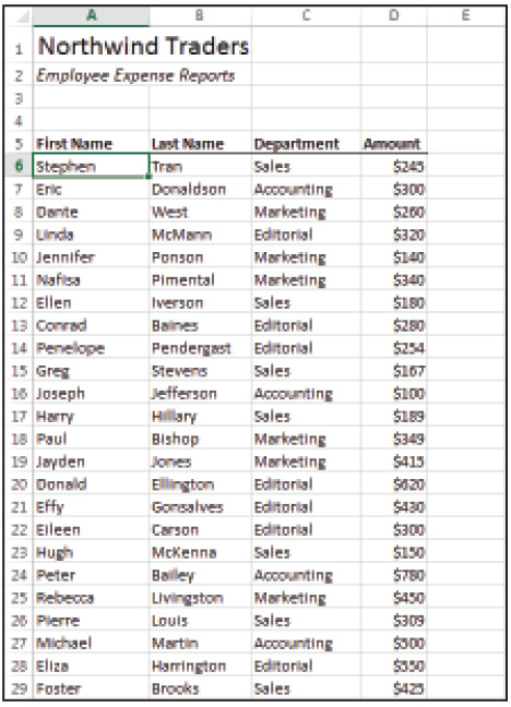
A list contains similar sets of data.

Creating a list

Creating a list is very simple. The first step is to determine the categories of information that you want to capture, and then enter a label in each column of the list. For instance, you could have a file with information about your sales force, where the columns are labeled First Name, Last Name, Department, and Amount.

The row that contains the column headings or field names is referred to as the Header Row. The header row is important when you begin to work with your data, since it is used to specify fields to sort by or records to filter.

Adding records to a list

When creating a list, the first step is to create the header row; you can then enter records in the rows directly beneath.

To move to the next field in the list, press the Tab key on your keyboard. To move down the list, you can press the Enter key: Excel recognizes the data entry pattern as a list and automatically moves the cell pointer to the first field in the next row.

Here’s an exercise for you to practice creating lists in Excel.

1 Open Excel, choose File > Open and navigate to the Excel06lessons folder. Open the file named excel06_list.

2 Choose File > Save As and navigate to the Excel06lessons folder again. Name the file excel06_list_work.

3 Click in cell A38 and type James.

4 Press Tab and type Gilford in cell B38.

5 Press Tab and type Sales in cell C38. Notice that when you begin typing Sales, Excel automatically fills in the remainder for you with its AutoComplete feature.

6 Press Tab and type 345 in cell D38.

7 Press Enter to move to cell A39.

8 Save the file, but don’t close it; you’ll use it in the next section.

When you press the Enter key, Excel moves the cell pointer to the next record.

Sorting records

Excel enables you to organize the data in a list to suit your needs. You can sort the data so it appears in a certain order, either alphabetically or numerically, and in ascending or descending order. You can also create a custom sort to arrange records on multiple fields.

For all four exercises in this section, use the same exercise file you used in the previous section. Don’t close the file at the end of each exercise.

Sorting records in ascending order

To sort records in ascending order:

1 Position the cell pointer in cell B6 to sort the records by Last Name.

2 From the Data tab, choose Sort A to Z. Excel sorts the list alphabetically by last name.

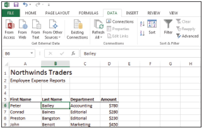
Sort records in a list to rearrange the order alphabetically.

Sorting records in descending order

To sort records in descending order:

1 Position the cell pointer in cell D6 to sort by the Amount field.

2 From the Data tab, choose Sort Z to A. Excel sorts the list from highest to lowest by the Amount field.

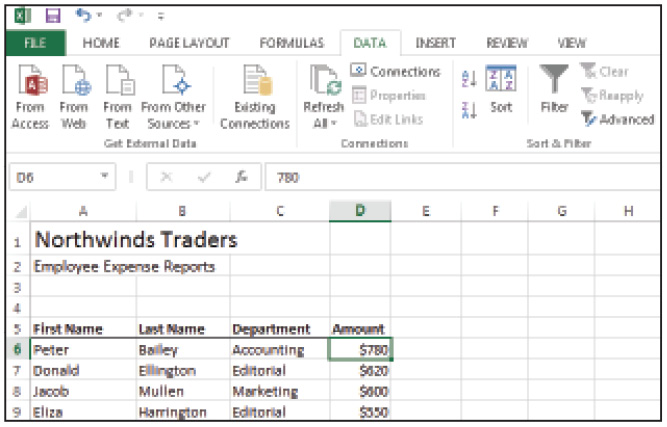
Sort numeric values in a list in descending order to rearrange the order from highest to lowest.

Sorting selected records

You can also sort a subset of records rather than the entire list. When you sort a select group and choose the Sort A to Z or Sort Z to A commands, Excel automatically sorts by the first field in the list. To sort by a different field you must use the Sort command.

1 Select range A6:E16.

2 From the Data tab, choose Sort.

3 In the Sort By field, select Last Name.

4 Change the Order to A to Z and click OK.

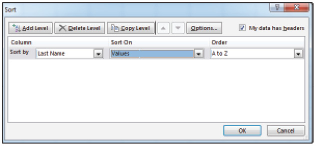
Sort a subset of records with the Sort command.

Creating a custom sort

When you want to sort records by more than one field, (for instance, by Department and then Last Name), you can create a custom sort.

1 Position the cell pointer in cell A6.

2 From the Data tab, choose Sort; then, select Department in the Sort By field.

3 Click the Add Level button.

4 In the Then By field, select Last Name, and then click OK. The data is now sorted alphabetically by the department and then alphabetically by the last name.

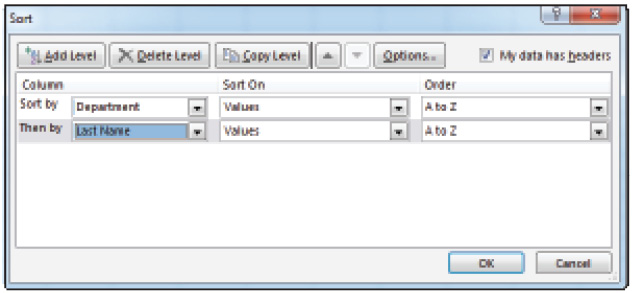
With the Sort command, you can sort records by more than one field.

Sort records by more than one field when you want view records by multiple order.

5 Save the file, but don’t close it; you’ll use it in the next section.

Filtering records

By filtering records, you can select the records to view in your list. Filtering records is similar to sorting in that you indicate the field by which you want to filter. You can also create multiple levels of filtering so you can view records by more than one criterion. For example, you can view records by specific departments or by a certain amount. When you apply a filter, Excel hides the records that do not meet the filter.

For all exercises in this section, use the same exercise file you have been using till now. Don’t close the file at the end of each exercise.

Creating a filter

To create a filter:

1 Position the cell pointer in cell A6.

2 From the Data tab, choose Filter. Excel adds filter buttons to the field names in row 5 in your list.

3 Click the Department filter button.

4 Click Select All to deselect it; select Marketing.

Filtering allows you to designate the records you want to view.

5 Click OK. Excel displays only the records from the Marketing department.

Filtered records only display the records containing the filter you specified.

Clearing a filter

Excel indicates when a filter is in place by adding the filter symbol to the field heading you are filtering by. When you hover the pointer over the field heading, a box pops up telling you the current filter that is in place.

1 Click in cell A20.

2 From the Sort & Filter group in the Data tab, choose Clear. Excel redisplays all the records in the list.

Custom filtering

You can define a custom filter when the data must meet specific criteria. For instance, you can locate records that fall within a certain range of values or contain a certain string of text.

1 Position the cell pointer in cell A6.

2 From the Data tab, make sure Filter is selected.

3 Click the Amount filter, select Number Filters, and then choose Greater Than.

4 In the Custom AutoFilter dialog box, type 400 in the box adjacent to is greater than.

AutoFilters let you search for specific records.

5 Click OK to only show records that have amounts over $400.

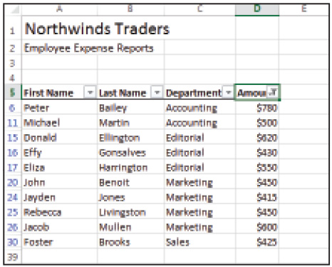
Filtered records display only those where the amount is greater than $400.

6 Save the file, but don’t close it; you’ll use it in the next section.

Searching records

To quickly find records in your list, use the Search feature.

1 Click in cell A6.

2 From the Data tab, click Filter twice. Excel removes the last filter setting and then adds filter buttons to the field names in your list again and removes the current filter.

3 Click the Last Name filter.

4 In the Search box, type Gonsalves and click OK. Excel displays only those records that meet the specified search criteria.

Find specific records with the Search filter.

5 Save the file, but don’t close it; you’ll use it in the next section.

Deleting records

When you need to delete records from a list, you can delete them directly from the worksheet, just as you would any data you no longer need. If you’re working with a large list, you should first filter the list to display only those records you want to delete. Use the Delete command to remove the filtered records from the list.

1 Click in cell A16.

2 From the Data tab, click Filter twice to clear the previous filter settings and begin a new filter.

3 Click the Department filter.

4 Click Select All to deselect it and choose Accounting.

5 Click OK. Excel filters the list to display only those records from the Accounting department.

6 Highlight range A6:E11 and in the Cells group on the Home tab, choose Delete.

7 Click OK when prompted to delete the rows. Excel removes the records from the Accounting department. Click the Undo button to restore the deleted records.

Delete filtered records from a list with the Delete command.

8 Click the Filter button on the Data tab to clear the current filter.

9 Save the file, but don’t close it; you’ll use it in the next section.

Removing duplicates

Excel can scan a list and search for duplicate entries. If it finds any, you can instruct Excel to remove them from the list.

1 Click in cell A6.

2 From the Data tab, choose Remove Duplicates.

3 Click the Unselect All button.

4 From the Columns section of Remove Duplicates dialog box, select First Name and Last Name.

Remove records that contain duplicate values.

5 Click OK. If there were records with duplicate first name and last name entries, they would be removed.

6 In the resulting dialog box, click OK to acknowledge that no duplicate values were found.

Extracting records

Organizing data in a list is very important, and so is pulling data out when needed. With Advanced sort, you can pull data from a list and store it in another area of the worksheet. By extracting specific records, we can analyze a subset of the data.

Before you can use the Advanced Sort feature, you must define a criteria range in the worksheet. The criteria range is identical to the header row in the list in that it contains a copy of the field names used in the list. To define the criteria, enter the data or criteria you want to find immediately below each column heading. You can indicate that the records be copied to another location for further analysis.

Defining the criteria range

To define the criteria range:

1 Select range A5:D5 and choose Copy from the Home tab.

2 Click in cell G5 and press Enter to paste the copied headings.

3 In cell J6, enter >400.

Extracting records defined in the criteria range

To extract the records you defined in the criteria range:

1 Click in cell L5.

2 From the Sort & Filter group of the Data tab, choose Advanced. Excel automatically selects range A5:D38 as the List range.

3 Change Excel’s automatic selection to indicate range G5:J6 as the Criteria range.

4 Select Copy to Another Location.

5 Indicate cell L5 as the Copy to range.

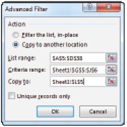
Use Advanced Filter to extract a range of records from a list.

6 Click OK. Excel pulls the records that match the criteria and copies them over under cell L5.

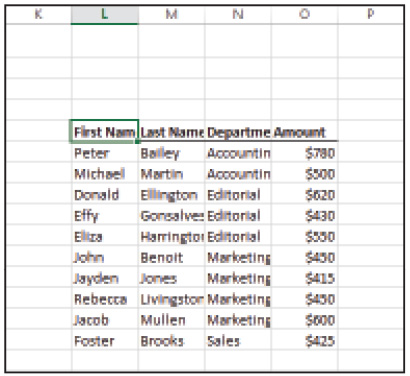
Extract a range of records for further analysis.

7 Save the file, but don’t close it; you’ll use it in the next section.

Subtotaling data

Excel’s Subtotal command allows you to summarize data in your lists by calculating subtotal and grand total amounts for numeric fields. When you summarize a list in such a manner, Excel calculates subtotals on subsets of data. For example, you can quickly determine sales revenue by department or determine the average number of units sold by branch.

Prior to adding subtotals, you must sort the list by the appropriate field.

1 Click in cell C6.

2 From the Home tab, choose Sort A to Z. Excel sorts the list by department if this was not already done.

Adding subtotals

To add subtotals:

1 Click in cell A6.

2 From the Outline group on the Data tab, choose Subtotal.

3 From the At each change in drop-down menu, select Department.

4 In the Add subtotal to box, select Amount.

You can add subtotal amounts at each change in Department.

5 Click OK. Subtotals are now added to the list below each department.

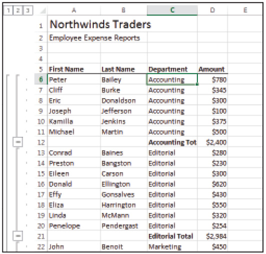
Subtotal amounts are added to the list.

Grouping records

When Subtotals are added to an Excel list, each set of records is automatically grouped on the field by which they are subtotaled. When records are grouped in such a way, you can collapse the details of the group to display the subtotals only, and you can expand each group to display the detailed data.

Excel automatically applies an outline view to the worksheet list after subtotals are added. This view offers you single-click access to hiding and expanding details. You can collapse and expand outline levels with the Outline symbols or with the Show Detail and Hide Detail commands from the Data tab.

Hiding and showing details

1 Click in cell C7 and choose Hide Detail () from the Data tab. Excels hides rows 6 through 11 and displays the Subtotal amount for the Accounting department in row 12.

Departmental details have been hidden in the Outline view to display Subtotal data only.

2 Choose Show Detail () to expand the detail items for the Accounting group; in this case, rows 6 through 11.

Click the Level 1 symbol to hide all details and display the Grand Total amount only. Click the Level 2 symbol to show subtotal amounts for each group. Click the Level 3 symbol to display all detail data.

Removing an outline

You can remove the outline from your worksheet list without removing the subtotal and grand total calculations. However, prior to removing the outline, make sure you expand the outline to include all your worksheet data. The quickest way to do this is to click the lowest level number displayed in your outline. For the exercise file you’ve been using throughout this lesson, this would be Level 3.

1 Click the drop-down arrow under the Ungroup button from the Data tab.

2 Select Clear Outline. Excel clears the outline from the display and retains the subtotal rows and data.

3 Choose Subtotal from the Data tab and click OK to add the Outline back to the list. Choose Subtotal and click Remove All from the resulting Subtotal dialog box. Excel removes both the outline and subtotals from the list.

4 Save the file, but don’t close it; you’ll use it in the next section.

Using data validation

Excel’s Data Validation tools enable you to restrict the type of data that users enter into the field of a list. By doing so, you can streamline data entry and ensure that the data meets a certain level of authentication. Data Validation can also help cut down on data entry errors. For instance, you can create a list of choices from which users can make a selection for a field such as Department. Or impose a restriction on the highest amount that can be entered into a field that captures expense-related items.

Creating data validation rules

To create data validation rules:

1 In cell E5, type Date Submitted and press Enter.

2 Select range E6:E38 and click Data Validation in the Data tab.

3 Select Date in the Allow field; select between in the Data field.

4 Type 1/1/13 in the Start Date field; type 1/31/13 in the End Date field. Click OK.

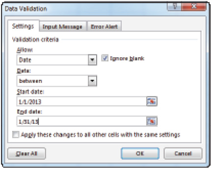
Restrict data entry to specific dates with Data Validation.

Entering data using data validation

To enter data using data validation:

1 Click in cell E6.

2 Type 1/2/13 and press Enter.

3 Type 1/4/13 in cell E7 and press Enter.

4 Type 2/2/13 in cell E8 and press Enter. Excel displays an error message alerting you that the value you entered is not valid.

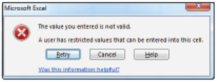
Error messages are displayed when a user breaks a Data Validation rule.

5 Click Cancel and enter 1/2/13 in cell E8 and press Enter.

Creating an input message

You can define the message that a user sees when the cell pointer moves to a range that has data validation enabled.

1 Select range E6:E38.

2 In the Data tab, choose Data Validation, and then click the Input Message tab.

3 Type Date Submitted in the Title field; type Enter dates for the current month only. in the Input message field.

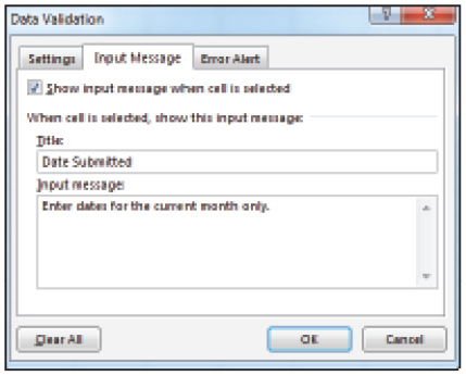
Define the message that users will see when they point to a cell with data validation rules.

4 Click OK. The custom message you created is displayed explaining the data validation rules.

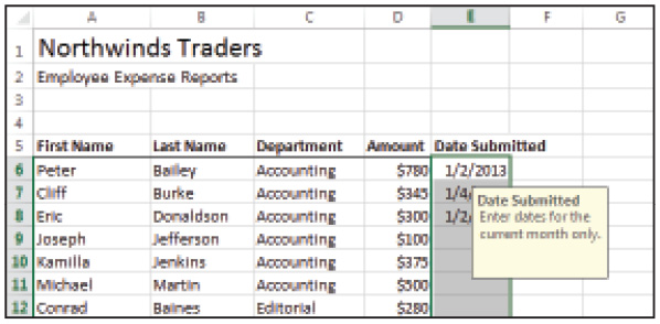
Define the message that users will see when they point to a cell with data validation rules.

Creating the error alert

In addition to creating a specialized message when users enter a cell using Data Validation, you can create a custom error message when users break the data entry rule.

1 Make sure range E6:E38.

2 In the Data tab, choose Data Validation.

3 Click the Error Alert tab and select Stop from the Style drop-down menu.

4 Type Invalid Date in the Title field; type Enter a date from the current month only. in the Error Message field.

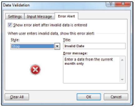
Create a custom error message for when users type the incorrect data.

5 Click OK. Test by typing 2/5/13 in cell E9 and press Enter.

A custom error message alerts the user to invalid entries.

6 Click Retry and type 1/5/13 and press Enter.

7 Choose File > Save and then File > Close.

Converting text to columns

Many times, the data we want to work with in an Excel list comes from other sources. To manipulate the information in the column and row worksheet structure of Excel, we need to clean up the data and convert it so that it can be more readily used.

For example, suppose that you import a mailing list that contains both the first and last name of the customer in the same field. In a list such as this, you can’t sort the records by last name. The best option is to split the complete name into two separate fields: First Name and Last Name.

To convert text into columnar form

Before you convert text into multiple columns, you must make sure that there are enough blank columns to hold the split data; otherwise, existing information will be overwritten.

In this exercise, you will begin by opening the practice file, save it, and rename it so you have your own working copy. Then you will add a blank column to your working copy so you have enough columns to hold the split data; and finally, you will split the data.

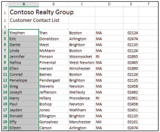
1 Choose File > Open and navigate to the Excel06lessons folder on your Computer. Open the file named excel06_customers.

2 Choose File > Save As and navigate back to the Excel06lessons folder. Name the file excel06_customers_work.

3 Click in column B and click the down arrow below Insert from the Home tab. Select Insert Sheet Columns.

4 Select range A4:A32 and choose Text to Columns from the Data tab.

5 In the Covert Text to Columns wizard, choose Delimited. Then, click Next.

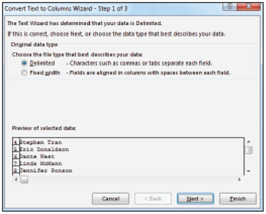
Convert text entries into multiple columns.

6 Select Space as the Delimiter and click Next. Click Finish. Excel splits the names from column A into first and last name entries in columns A and B.

Convert multi-word text entries into separate columns for easy manipulation.

7 Save the file, but don’t close it; you’ll use it in the next section.

Using Flash Fill

The Flash Fill command is another time-saving technique for working with data imported from other programs. Flash Fill evaluates a range of cells for any patterns or consistencies that it might find. When it senses a pattern, it automatically fills in the remainder of the data for you.

For example, in the following exercise, column A will contain the first and last name in the same field. We will use Flash Fill to fill column B with the first name and column C with the last name.

1 Click the Undo button two times to revert the worksheet you used in the previous exercise back to its original state.

2 Click in cell B4 and choose Insert > Insert Sheet Columns twice from the Home tab.

3 Click in cell B4 and type Stephen.

4 Click in cell B5 and type Eri. Excel senses the pattern and fills in the remainder of first names in column B. To accept the fill, press Enter.

Flash Fill cuts down on data entry by sensing patterns in your data.

5 Click in cell C4 and type Tran.

6 Click in cell C5 and type Dona. Again, Excel senses the pattern and fills in the remainder of last names in column C. Press Enter to accept the pattern.

7 Select range A4:A32 and choose Delete > Delete Cells from the Home tab.

8 Select Shift cells left and click OK. This removes the data in column A, which had become obsolete.

You’ve now completed Lesson 6. In our next lesson, “Using Templates,” you will learn how to use and customize the templates included in Excel 2013.

Self study

Complete the following Self study exercises using the excel06_list_work.

1 Using the Sort command, sort the records by Department in ascending order, Last Name in ascending order, and Amount in Descending order.

2 Filter the records so only those records with an Amount greater than $500 are displayed.

3 Using the Quick Analysis button tool, add Data Bars to the expense list.

Review

Questions

1 How do you sort records in alphabetical order?

2 What is the difference between sorting records and filtering records?

3 How do you remove records from a list?

4 How do you group records for subtotaling purposes?

5 How do you split data into multiple columns?

Answers

1 To sort records in alphabetical order, click in the column on your list that contains the data you want to sort by, and choose Sort A to Z from the Data tab.

2 The difference between sorting and filtering records is that, when you sort records, you rearrange the order by which the records are displayed in a list. When you filter records, you specify which records are displayed in a list.

3 Before removing records from a list, you should filter the records so only those you want to remove are displayed. Once you have displayed the records you want to delete, select the records and choose Delete Sheet Rows from the Home tab.

4 To generate subtotals for groups of records, first sort the list by the field you want to group by with the Data Sort command. Next, click in the column containing the sorted field and choose Subtotal from the Data tab.

5 To split data into multiple columns, insert a column to the immediate right of the column you want to split using Insert Sheet Columns from the Home tab. Then select the cells you want to split and choose Text to Columns from the Data tab.