
Chapter 4
Dimension-Reduction Methods
4.1 Need for Dimension-Reduction in Data Mining
The databases typically used in data mining may have millions of records and thousands of variables. It is unlikely that all of the variables are independent, with no correlation structure among them. Data analysts need to guard against multicollinearity, a condition where some of the predictor variables are strongly correlated with each other. Multicollinearity leads to instability in the solution space, leading to possible incoherent results, such as in multiple regression, where a multicollinear set of predictors can result in a regression which is significant overall, even when none of the individual variables is significant. Even if such instability is avoided, inclusion of variables which are highly correlated tends to overemphasize a particular component of the model, as the component is essentially being double counted.
Bellman1 noted that the sample size needed to fit a multivariate function grows exponentially with the number of variables. In other words, higher-dimension spaces are inherently sparse. For example, the empirical rule tells us that, in one-dimension, about 68% of normally distributed variates lie between one and negative one standard deviation from the mean; while, for a 10-dimension multivariate normal distribution, only 2% of the data lies within the analogous hypersphere.2
The use of too many predictor variables to model a relationship with a response variable can unnecessarily complicate the interpretation of the analysis, and violates the principle of parsimony, that one should consider keeping the number of predictors to such a size that would be easily interpreted. Also, retaining too many variables may lead to overfitting, in which the generality of the findings is hindered because new data do not behave the same as the training data for all the variables.
Further, analysis solely at the variable-level might miss the fundamental underlying relationships among the predictors. For example, several predictors might fall naturally into a single group, (a factor or a component), which addresses a single aspect of the data. For example, the variables savings account balance, checking account balance, home equity, stock portfolio value, and 401k balance might all fall together under the single component, assets.
In some applications, such as image analysis, retaining full dimensionality would make most problems intractable. For example, a face classification system based on ![]() pixel images could potentially require vectors of dimension 65,536.
pixel images could potentially require vectors of dimension 65,536.
Humans are innately endowed with visual pattern recognition abilities, which enable us in an intuitive manner to discern patterns in graphic images at a glance: the patterns that might elude us if presented algebraically or textually. However, even the most advanced data visualization techniques do not go much beyond five dimensions. How, then, can we hope to visualize the relationship among the hundreds of variables in our massive data sets?
Dimension-reduction methods have the goal of using the correlation structure among the predictor variables to accomplish the following:
- To reduce the number of predictor items.
- To help ensure that these predictor items are independent.
- To provide a framework for interpretability of the results.
In this chapter, we examine the following dimension-reduction methods:
- Principal components analysis (PCA)
- Factor analysis
- User-defined composites
This next section calls upon knowledge of matrix algebra. For those of you whose matrix algebra may be rusty, concentrate on the meaning of Results 1–3 (see below).3 Immediately after, we shall apply all of the following terminologies and notations in terms of a concrete example, using the real-world data.
4.2 Principal Components Analysis
PCA seeks to explain the correlation structure of a set of predictor variables, using a smaller set of linear combinations of these variables. These linear combinations are called components. The total variability of a data set produced by the complete set of m variables can often be mostly accounted for by a smaller set of k linear combinations of these variables, which would mean that there is almost as much information in the k components as there is in the original m variables. If desired, the analyst can then replace the original m variables with the k < m components, so that the working data set now consists of n records on k components, rather than n records on m variables. The analyst should note that PCA acts solely on the predictor variables, and ignores the target variable.
Suppose that the original variables ![]() form a coordinate system in m-dimensional space. The principal components represent a new coordinate system, found by rotating the original system along the directions of maximum variability.
form a coordinate system in m-dimensional space. The principal components represent a new coordinate system, found by rotating the original system along the directions of maximum variability.
When preparing to perform data reduction, the analyst should first standardize the data, so that the mean for each variable is zero, and the standard deviation is one. Let each variable ![]() represent an
represent an ![]() vector, where n is the number of records. Then, represent the standardized variable as the
vector, where n is the number of records. Then, represent the standardized variable as the ![]() vector
vector ![]() , where
, where ![]() ,
, ![]() is the mean of
is the mean of ![]() , and
, and ![]() is the standard deviation of
is the standard deviation of ![]() . In matrix notation, this standardization is expressed as
. In matrix notation, this standardization is expressed as ![]() , where the “−1” exponent refers to the matrix inverse, and
, where the “−1” exponent refers to the matrix inverse, and ![]() is a diagonal matrix (nonzero entries only on the diagonal); the
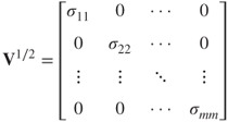
is a diagonal matrix (nonzero entries only on the diagonal); the ![]() standard deviation matrix is:
standard deviation matrix is:
Let ![]() refer to the symmetric covariance matrix:
refer to the symmetric covariance matrix:
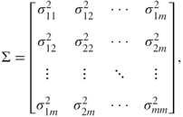
where ![]() refers to the covariance between
refers to the covariance between ![]() and
and ![]() .
.
The covariance is a measure of the degree to which two variables vary together. A positive covariance indicates that, when one variable increases, the other tends to increase, while a negative covariance indicates that, when one variable increases, the other tends to decrease. The notation ![]() is used to denote the variance of
is used to denote the variance of ![]() . If
. If ![]() and
and ![]() are independent, then
are independent, then ![]() ; but
; but ![]() does not imply that
does not imply that ![]() and
and ![]() are independent. Note that the covariance measure is not scaled, so that changing the units of measure would change the value of the covariance.
are independent. Note that the covariance measure is not scaled, so that changing the units of measure would change the value of the covariance.
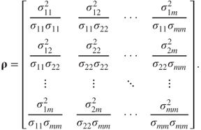
The correlation coefficient ![]() avoids this difficulty by scaling the covariance by each of the standard deviations:
avoids this difficulty by scaling the covariance by each of the standard deviations:

Then, the correlation matrix is denoted as ![]() (rho, the Greek letter for r):
(rho, the Greek letter for r):
Consider again the standardized data matrix ![]() . Then, as each variable has been standardized we have
. Then, as each variable has been standardized we have ![]() , where 0 denotes an
, where 0 denotes an ![]() matrix of zeroes, and Z has covariance matrix
matrix of zeroes, and Z has covariance matrix ![]() . Thus, for the standardized data set, the covariance matrix and the correlation matrix are the same.
. Thus, for the standardized data set, the covariance matrix and the correlation matrix are the same.
The ith principal component of the standardized data matrix ![]() is given by:
is given by: ![]() , where
, where ![]() refers to the ith eigenvector (discussed below), and
refers to the ith eigenvector (discussed below), and ![]() refers to the transpose of
refers to the transpose of ![]() . The principal components
. The principal components ![]() are linear combinations of the standardized variables in Z, such that (a) the variances of the
are linear combinations of the standardized variables in Z, such that (a) the variances of the ![]() are as large as possible, and (b) the
are as large as possible, and (b) the ![]() 's are uncorrelated.
's are uncorrelated.
The first principal component is the linear combination ![]() that has greater variability than any other possible linear combination of the Z variables. Thus,
that has greater variability than any other possible linear combination of the Z variables. Thus,
- the first principal component is the linear combination
 that maximizes
  ;
; - the second principal component is the linear combination
 that is independent of
  , and maximizes
  ;
; - in general, the ith principal component is the linear combination
 that is independent of all the other principal components
  , and maximizes
  .
.
Eigenvalues. Let B be an ![]() matrix, and let I be the
matrix, and let I be the ![]() identity matrix (diagonal matrix with 1's on the diagonal). Then the scalars (numbers of dimension
identity matrix (diagonal matrix with 1's on the diagonal). Then the scalars (numbers of dimension ![]() )
) ![]() are said to be the eigenvalues of B if they satisfy
are said to be the eigenvalues of B if they satisfy ![]() , where |Q| denotes the determinant of Q.
, where |Q| denotes the determinant of Q.
Eigenvectors. Let B be an ![]() matrix, and let
matrix, and let ![]() be an eigenvalue of B. Then nonzero
be an eigenvalue of B. Then nonzero ![]() vector e is said to be an eigenvector of B, if
vector e is said to be an eigenvector of B, if ![]() .
.
The following results are very important for our PCA analysis.
- Result 1
The total variability in the standardized set of predictors equals the sum of the variances of the Z-vectors, which equals the sum of the variances of the components, which equals the sum of the eigenvalues, which equals the number of predictors. That is,
- Result 2
The partial correlation between a given component and a given predictor variable is a function of an eigenvector and an eigenvalue. Specifically,
 , where
  are the eigenvalue–eigenvector pairs for the correlation matrix
  , and we note that
  . In other words, the eigenvalues are ordered by size. (A partial correlation coefficient is a correlation coefficient that takes into account the effect of all the other variables.)
 - Result 3
The proportion of the total variability in Z that is explained by the ith principal component is the ratio of the ith eigenvalue to the number of variables, that is, the ratio
 .
.
Next, to illustrate how to apply PCA on real data, we turn to an example.
4.3 Applying PCA to the Houses Data Set
We turn to the Houses data set,4 which provides census information from all the block groups from the 1990 California census. For this data set, a block group has an average of 1425.5 people living in an area that is geographically compact. Block groups were excluded that contained zero entries for any of the variables. Median house value is the response variable; the predictor variables are the following:
| Median income | Population |
| Housing median age | Households |
| Total rooms | Latitude |
| Total bedrooms | Longitude |
The original data set had 20,640 records, of which 18,540 were randomly selected for a training data set, and 2100 held out for a test data set. A quick look at the variables is provided in Figure 4.1. (“Range” indicates IBM Modeler's type label for continuous variables.)

Figure 4.1 A quick look at the houses data set.
Median house value appears to be in dollars, but median income has been scaled to a 0–15 continuous scale. Note that longitude is expressed in negative terms, meaning west of Greenwich. Larger absolute values for longitude indicate geographic locations further west.
Relating this data set to our earlier notation, we have ![]() = median income,
= median income, ![]() = housing median age,
= housing median age, ![]() ,
, ![]() = longitude, so that m = 8, and n = 18,540. A glimpse of the first 20 records in the training data set looks like Figure 4.2. So, for example, for the first block group, the median house value is $425,600, the median income is 8.3252 (on the census scale), the housing median age is 41, the total rooms is 880, the total bedrooms is 129, the population is 322, the number of households is 126, the latitude is 37.88 north, and the longitude is 122.23 west. Clearly, this is a smallish block group with high median house value. A map search reveals that this block group is centered between the University of California at Berkeley and Tilden Regional Park.
= longitude, so that m = 8, and n = 18,540. A glimpse of the first 20 records in the training data set looks like Figure 4.2. So, for example, for the first block group, the median house value is $425,600, the median income is 8.3252 (on the census scale), the housing median age is 41, the total rooms is 880, the total bedrooms is 129, the population is 322, the number of households is 126, the latitude is 37.88 north, and the longitude is 122.23 west. Clearly, this is a smallish block group with high median house value. A map search reveals that this block group is centered between the University of California at Berkeley and Tilden Regional Park.

Figure 4.2 A glimpse of the first twenty records in the houses data set.
Note from Figure 4.1 the great disparity in variability among the predictors. The median income has a standard deviation less than 2, while the total rooms has a standard deviation over 2100. If we proceeded to apply PCA without first standardizing the variables, total rooms would dominate median income's influence, and similarly across the spectrum of variabilities. Therefore, standardization is called for. The variables were standardized, and the Z-vectors found, ![]() , using the means and standard deviations from Figure 4.1.
, using the means and standard deviations from Figure 4.1.
Note that normality of the data is not strictly required to perform non-inferential PCA (Johnson and Wichern, 2006),5 but that strong departures from normality may diminish the observed correlations (Hair et al., 2006).6 As data mining applications usually do not involve inference, we will not worry about normality.
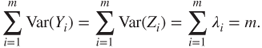
Next, we examine the matrix plot of the predictors in Figure 4.3 to explore whether correlations exist. Diagonally from left to right, we have the standardized variables minc_z (median income), hage_z (housing median age), rooms_z (total rooms), bedrms_z (total bedrooms), popn_z (population), hhlds_z (number of households), lat_z (latitude), and long_z (longitude). What does the matrix plot tell us about the correlation among the variables? Rooms, bedrooms, population, and households all appear to be positively correlated. Latitude and longitude appear to be negatively correlated. (What does the plot of latitude vs longitude look like? Did you say the State of California?) Which variable appears to be correlated the least with the other predictors? Probably housing median age. Table 4.1 shows the correlation matrix ![]() for the predictors. Note that the matrix is symmetrical, and that the diagonal elements all equal one. A matrix plot and the correlation matrix are two ways of looking at the same thing: the correlation structure among the predictor variables. Note that the cells for the correlation matrix
for the predictors. Note that the matrix is symmetrical, and that the diagonal elements all equal one. A matrix plot and the correlation matrix are two ways of looking at the same thing: the correlation structure among the predictor variables. Note that the cells for the correlation matrix ![]() line up one-to-one with the graphs in the matrix plot.
line up one-to-one with the graphs in the matrix plot.
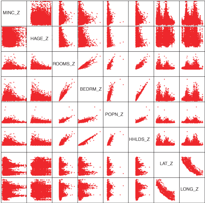
Figure 4.3 Matrix plot of the predictor variables.
Table 4.1 The correlation matrix ![]()
| Correlations | ||||||||
| MINC_Z | HAGE_Z | ROOMS_Z | BEDRMS_Z | POPN_Z | HHLDS_Z | LAT_Z | LONG_Z | |
| MINC_Z | 1.000 | −0.117 | 0.199 | −0.012 | 0.002 | 0.010 | −0.083 | −0.012 |
| HAGE_Z | −0.117 | 1.000 | −0.360 | −0.318 | −0.292 | −0.300 | 0.011 | −0.107 |
| ROOMS_Z | 0.199 | −0.360 | 1.000 | 0.928 | 0.856 | 0.919 | −0.035 | 0.041 |
| BEDRMS_Z | −0.012 | −0.318 | 0.928 | 1.000 | 0.878 | 0.981 | −0.064 | 0.064 |
| POPN_Z | 0.002 | −0.292 | 0.856 | 0.878 | 1.000 | 0.907 | −0.107 | 0.097 |
| HHLDS_Z | 0.010 | −0.300 | 0.919 | 0.981 | 0.907 | 1.000 | −0.069 | 0.051 |
| LAT_Z | −0.083 | 0.011 | −0.035 | −0.064 | −0.107 | −0.069 | 1.000 | −0.925 |
| LONG_Z | −0.012 | −0.107 | 0.041 | 0.064 | 0.097 | 0.051 | −0.925 | 1.000 |
What would happen if we performed, say, a multiple regression analysis of median housing value on the predictors, despite the strong evidence for multicollinearity in the data set? The regression results would become quite unstable, with (among other things) tiny shifts in the predictors leading to large changes in the regression coefficients. In short, we could not use the regression results for profiling.
This is where PCA comes in. PCA can sift through the correlation structure, and identify the components underlying the correlated variables. Then, the principal components can be used for further analysis downstream, such as in regression analysis, classification, and so on.
PCA was carried out on the eight predictors in the house data set. The component matrix is shown in Table 4.2. Each of the columns in Table 4.2 represents one of the components ![]() . The cell entries are called the component weights, and represent the partial correlation between the variable and the component. Result 2 tells us that these component weights therefore equal
. The cell entries are called the component weights, and represent the partial correlation between the variable and the component. Result 2 tells us that these component weights therefore equal ![]() , a product involving the ith eigenvector and eigenvalue. As the component weights are correlations, they range between one and negative one.
, a product involving the ith eigenvector and eigenvalue. As the component weights are correlations, they range between one and negative one.
Table 4.2 The component matrix
| Component Matrixa | ||||||||
| Component | ||||||||
| 1 | 2 | 3 | 4 | 5 | 6 | 7 | 8 | |
| MINC_Z | 0.086 | −0.058 | 0.922 | 0.370 | −0.02 | −0.018 | 0.037 | −0.004 |
| HAGE_Z | −0.429 | 0.025 | −0.407 | 0.806 | 0.014 | 0.026 | 0.009 | −0.001 |
| ROOMS_Z | 0.956 | 0.100 | 0.102 | 0.104 | 0.120 | 0.162 | −0.119 | 0.015 |
| BEDRMS_Z | 0.970 | 0.083 | −0.121 | 0.056 | 0.144 | −0.068 | 0.051 | −0.083 |
| POPN_Z | 0.933 | 0.034 | −0.121 | 0.076 | −0.327 | 0.034 | 0.006 | −0.015 |
| HHLDS_Z | 0.972 | 0.086 | −0.113 | 0.087 | 0.058 | −0.112 | 0.061 | 0.083 |
| LAT_Z | −0.140 | 0.970 | 0.017 | −0.088 | 0.017 | 0.132 | 0.113 | 0.005 |
| LONG_Z | 0.144 | −0.969 | −0.062 | −0.063 | 0.037 | 0.136 | 0.109 | 0.007 |
Extraction method: Principal component analysis.
a Eight components extracted.
In general, the first principal component may be viewed as the single best summary of the correlations among the predictors. Specifically, this particular linear combination of the variables accounts for more variability than any other linear combination. It has maximized the variance ![]() . As we suspected from the matrix plot and the correlation matrix, there is evidence that total rooms, total bedrooms, population, and households vary together. Here, they all have very high (and very similar) component weights, indicating that all four variables are highly correlated with the first principal component.
. As we suspected from the matrix plot and the correlation matrix, there is evidence that total rooms, total bedrooms, population, and households vary together. Here, they all have very high (and very similar) component weights, indicating that all four variables are highly correlated with the first principal component.
Let us examine Table 4.3, which shows the eigenvalues for each component, along with the percentage of the total variance explained by that component. Recall that Result 3 showed us that the proportion of the total variability in Z that is explained
Table 4.3 Eigenvalues and proportion of variance explained by each component
| Initial Eigenvalues | |||
| Component | Total | % of Variance | Cumulative% |
| 1 | 3.901 | 48.767 | 48.767 |
| 2 | 1.910 | 23.881 | 72.648 |
| 3 | 1.073 | 13.409 | 86.057 |
| 4 | 0.825 | 10.311 | 96.368 |
| 5 | 0.148 | 1.847 | 98.215 |
| 6 | 0.082 | 1.020 | 99.235 |
| 7 | 0.047 | 0.586 | 99.821 |
| 8 | 0.014 | 0.179 | 100.000 |
by the ith principal component is ![]() , the ratio of the ith eigenvalue to the number of variables. Here, we see that the first eigenvalue is 3.901, and as there are eight predictor variables, this first component explains
, the ratio of the ith eigenvalue to the number of variables. Here, we see that the first eigenvalue is 3.901, and as there are eight predictor variables, this first component explains ![]() of the variance, as shown in Table 4.3 (allowing for rounding). So, a single component accounts for nearly half of the variability in the set of eight predictor variables, meaning that this single component by itself carries about half of the information in all eight predictors. Notice also that the eigenvalues decrease in magnitude,
of the variance, as shown in Table 4.3 (allowing for rounding). So, a single component accounts for nearly half of the variability in the set of eight predictor variables, meaning that this single component by itself carries about half of the information in all eight predictors. Notice also that the eigenvalues decrease in magnitude, ![]() ,
, ![]() , as we noted in Result 2.
, as we noted in Result 2.
The second principal component ![]() is the second-best linear combination of the variables, on the condition that it is orthogonal to the first principal component. Two vectors are orthogonal if they are mathematically independent, have no correlation, and are at right angles to each other. The second component is derived from the variability that is left over, once the first component has been accounted for. The third component is the third-best linear combination of the variables, on the condition that it is orthogonal to the first two components. The third component is derived from the variance remaining after the first two components have been extracted. The remaining components are defined similarly.
is the second-best linear combination of the variables, on the condition that it is orthogonal to the first principal component. Two vectors are orthogonal if they are mathematically independent, have no correlation, and are at right angles to each other. The second component is derived from the variability that is left over, once the first component has been accounted for. The third component is the third-best linear combination of the variables, on the condition that it is orthogonal to the first two components. The third component is derived from the variance remaining after the first two components have been extracted. The remaining components are defined similarly.
4.4 How Many Components Should We Extract?
Next, recall that one of the motivations for PCA was to reduce the number of distinct explanatory elements. The question arises, “How do we determine how many components to extract?” For example, should we retain only the first principal component, as it explains nearly half the variability? Or, should we retain all eight components, as they explain 100% of the variability? Well, clearly, retaining all eight components does not help us to reduce the number of distinct explanatory elements. As usual, the answer lies somewhere between these two extremes. Note from Table 4.3 that the eigenvalues for several of the components are rather low, explaining less than 2% of the variability in the Z-variables. Perhaps these would be the components we should consider not retaining in our analysis?
The criteria used for deciding how many components to extract are the following:
- The Eigenvalue Criterion
- The Proportion of Variance Explained Criterion
- The Minimum Communality Criterion
- The Scree Plot Criterion.
4.4.1 The Eigenvalue Criterion
Recall from Result 1 that the sum of the eigenvalues represents the number of variables entered into the PCA. An eigenvalue of 1 would then mean that the component would explain about “one variable's worth” of the variability. The rationale for using the eigenvalue criterion is that each component should explain at least one variable's worth of the variability, and therefore, the eigenvalue criterion states that only components with eigenvalues greater than 1 should be retained. Note that, if there are fewer than 20 variables, the eigenvalue criterion tends to recommend extracting too few components, while, if there are more than 50 variables, this criterion may recommend extracting too many. From Table 4.3, we see that three components have eigenvalues greater than 1, and are therefore retained. Component 4 has an eigenvalue of 0.825, which is not too far from one, so that we may decide to consider retaining this component as well, if other criteria support such a decision, especially in view of the tendency of this criterion to recommend extracting too few components.
4.4.2 The Proportion of Variance Explained Criterion
First, the analyst specifies how much of the total variability that he or she would like the principal components to account for. Then, the analyst simply selects the components one by one until the desired proportion of variability explained is attained. For example, suppose we would like our components to explain 85% of the variability in the variables. Then, from Table 4.3, we would choose components 1–3, which together explain 86.057% of the variability. However, if we wanted our components to explain 90% or 95% of the variability, then we would need to include component 4 along with components 1–3, which together would explain 96.368% of the variability. Again, as with the eigenvalue criterion, how large a proportion is enough?
This question is akin to asking how large a value of ![]() (coefficient of determination) is enough in the realm of linear regression. The answer depends in part on the field of study. Social scientists may be content for their components to explain only 60% or so of the variability, as human response factors are so unpredictable, while natural scientists might expect their components to explain 90–95% of the variability, as their measurements are often less variable. Other factors also affect how large a proportion is needed. For example, if the principal components are being used for descriptive purposes only, such as customer profiling, then the proportion of variability explained may be a shade lower than otherwise. However, if the principal components are to be used as replacements for the original (standardized) data set, and used for further inference in models downstream, then the proportion of variability explained should be as much as can conveniently be achieved, given the constraints of the other criteria.
(coefficient of determination) is enough in the realm of linear regression. The answer depends in part on the field of study. Social scientists may be content for their components to explain only 60% or so of the variability, as human response factors are so unpredictable, while natural scientists might expect their components to explain 90–95% of the variability, as their measurements are often less variable. Other factors also affect how large a proportion is needed. For example, if the principal components are being used for descriptive purposes only, such as customer profiling, then the proportion of variability explained may be a shade lower than otherwise. However, if the principal components are to be used as replacements for the original (standardized) data set, and used for further inference in models downstream, then the proportion of variability explained should be as much as can conveniently be achieved, given the constraints of the other criteria.
4.4.3 The Minimum Communality Criterion
For now, we postpone discussion of this criterion until we introduce the concept of communality below.
4.4.4 The Scree Plot Criterion
A scree plot is a graphical plot of the eigenvalues against the component number. Scree plots are useful for finding an upper bound (maximum) for the number of components that should be retained. See Figure 4.4 for the scree plot for this example. Most scree plots look broadly similar in shape, starting high on the left, falling rather quickly, and then flattening out at some point. This is because the first component usually explains much of the variability, the next few components explain a moderate amount, and the latter components only explain a small amount of the variability. The scree plot criterion is this: The maximum number of components that should be extracted is just before where the plot first begins to straighten out into a horizontal line. (Sometimes, the curve in a scree plot is so gradual that no such elbow point is evident; in that case, turn to the other criteria.) For example, in Figure 4.4, the plot straightens out horizontally starting at component 5. The line is nearly horizontal because the components all explain approximately the same amount of variance, which is not much. Therefore, the scree plot criterion would indicate that the maximum number of components we should extract is four, as the fourth component occurs just before where the line first begins to straighten out.
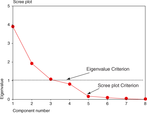
Figure 4.4 Scree plot. Stop extracting components before the line flattens out.
To summarize, the recommendations of our criteria are as follows:
- The Eigenvalue Criterion:
- Retain components 1–3, but do not throw away component 4 yet.
- The Proportion of Variance Explained Criterion
- Components 1–3 account for a solid 86% of the variability, and tacking on component 4 gives us a superb 96% of the variability.
- The Scree Plot Criterion
- Do not extract more than four components.
So, we will extract at least three but no more than four components. Which is it to be, three or four? As in much of data analysis, there is no absolute answer in this case to the question of how many components to extract. This is what makes data mining an art as well as a science, and this is another reason why data mining requires human direction. The data miner or data analyst must weigh all the factors involved in a decision, and apply his or her judgment, tempered by experience.
In a case like this, where there is no clear-cut best solution, why not try it both ways and see what happens? Consider Tables 4.4a and 4.4b, which compares the component matrices when three and four components are extracted, respectively. The component weights smaller than 0.15 are suppressed to ease the component interpretation. Note that the first three components are each exactly the same in both cases, and each is the same as when we extracted all eight components, as shown in Table 4.2 above (after suppressing the small weights). This is because each component extracts its portion of the variability sequentially, so that later component extractions do not affect the earlier ones.
Table 4.4a Component matrix for extracting three components
| Component Matrixa | |||
| Component | |||
| 1 | 2 | 3 | |
| MINC_Z | 0.922 | ||
| HAGE_Z | −0.429 | −0.407 | |
| ROOMS_Z | 0.956 | ||
| BEDRMS_Z | 0.970 | ||
| POPN_Z | 0.933 | ||
| HHLDS_Z | 0.972 | ||
| LAT_Z | 0.970 | ||
| LONG_Z | −0.969 | ||
Extraction method: PCA.
a Three components extracted.
Table 4.4b Component matrix for extracting four components
| Component Matrixa | ||||
| Component | ||||
| 1 | 2 | 3 | 4 | |
| MINC_Z | 0.922 | 0.370 | ||
| HAGE_Z | −0.429 | −0.407 | 0.806 | |
| ROOMS_Z | 0.956 | |||
| BEDRMS_Z | 0.970 | |||
| POPN_Z | 0.933 | |||
| HHLDS_Z | 0.972 | |||
| LAT_Z | 0.970 | |||
| LONG_Z | −0.969 | |||
Extraction method: PCA.
a Four components extracted.
4.5 Profiling the Principal Components
The client may be interested in detailed profiles of the principal components the analyst has uncovered. Let us now examine the salient characteristics of each principal component, giving each component a title for ease of interpretation.
- The Size Component. Principal component 1, as we saw earlier, is largely composed of the “block-group-size”-type variables, total rooms, total bedrooms, population, and households, which are all either large or small together. That is, large block groups have a strong tendency to have large values for all four variables, while small block groups tend to have small values for all four variables. Median housing age is a smaller, lonely counterweight to these four variables, tending to be low (recently built housing) for large block groups, and high (older, established housing) for smaller block groups.
- The Geographical Component. Principal component 2 is a “geographical” component, composed solely of the latitude and longitude variables, which are strongly negatively correlated, as we can tell by the opposite signs of their component weights. This supports our earlier exploratory data analysis (EDA) regarding these two variables in Figure 4.3 and Table 4.1. The negative correlation is because of the way latitude and longitude are signed by definition, and because California is broadly situated from northwest to southeast. If California was situated from northeast to southwest, then latitude and longitude would be positively correlated.
- Income and Age 1. Principal component 3 refers chiefly to the median income of the block group, with a smaller effect due to the housing median age of the block group. That is, in the data set, high median income is associated with more recently built housing, while lower median income is associated with older housing.
- Income and Age 2. Principal component 4 is of interest, because it is the one that we have not decided whether or not to retain. Again, it focuses on the combination of housing median age and median income. Here, we see that, once the negative correlation between these two variables has been accounted for, there is left over a positive relationship between these variables. That is, once the association between, for example, high incomes and recent housing has been extracted, there is left over some further association between higher incomes and older housing.
To further investigate the relationship between principal components 3 and 4, and their constituent variables, we next consider factor scores. Factor scores are estimated values of the factors for each observation, and are based on factor analysis, discussed in the next section. For the derivation of factor scores, see Johnson and Wichern.7
Consider Figure 4.5, which provides two matrix plots. The matrix plot on the left displays the relationships among median income, housing median age, and the factor scores for component 3, while the matrix plot on the right displays the relationships among median income, housing median age, and the factor scores for component 4. Tables 4.4 and 4.5 showed that components 3 and 4 both included each of these variables as constituents. However, there seemed to be a large difference in the absolute component weights, as for example, 0.922 having a greater amplitude than −0.407 for the component 3 component weights. Is this difference in magnitude reflected in the matrix plots?
Figure 4.5 Correlations between components 3 and 4, and their variables.
Consider the left side of Figure 4.5. The strong positive correlation between component 3 and median income is strikingly evident, reflecting the 0.922 positive correlation. But the relationship between component 3 and housing median age is rather amorphous. It would be difficult to estimate the correlation between component 3 and housing median age as being −0.407, with only the scatter plot to guide us. Similarly for the right side of Figure 4.5, the relationship between component 4 and housing median age is crystal clear, reflecting the 0.806 positive correlation, while the relationship between component 3 and median income is not entirely clear, reflecting its lower positive correlation of 0.370. We conclude, therefore, that the component weight of −0.407 for housing median age in component 3 is not of practical significance, and similarly for the component weight for median income in component 4.
This discussion leads us to the following criterion for assessing the component weights. For a component weight to be considered of practical significance, it should exceed ![]() in magnitude. Note that the component weight represents the correlation between the component and the variable; thus, the squared component weight represents the amount of the variable's total variability that is explained by the component. Thus, this threshold value of
in magnitude. Note that the component weight represents the correlation between the component and the variable; thus, the squared component weight represents the amount of the variable's total variability that is explained by the component. Thus, this threshold value of ![]() requires that at least 25% of the variable's variance be explained by a particular component.
requires that at least 25% of the variable's variance be explained by a particular component.
Table 4.5 therefore presents the component matrix from Tables 4.4a and 4.4b, this time suppressing the component weights below ![]() in magnitude. The component profiles should now be clear, and uncluttered:
in magnitude. The component profiles should now be clear, and uncluttered:
- The Size Component. Principal component 1 represents the “block group size” component, consisting of four variables: total rooms, total bedrooms, population, and households.
- The Geographical Component. Principal component 2 represents the “geographical” component, consisting of two variables: latitude and longitude.
- Median Income. Principal component 3 represents the “income” component, and consists of only one variable: median income.
- Housing Median Age. Principal component 4 represents the “housing age” component, and consists of only one variable: housing median age.
Table 4.5 Component matrix of component weights, suppressing magnitudes below ±0.50
| Component Matrixa | ||||
| Component | ||||
| 1 | 2 | 3 | 4 | |
| MINC_Z | 0.922 | |||
| HAGE_Z | 0.806 | |||
| ROOMS_Z | 0.956 | |||
| BEDRMS_Z | 0.970 | |||
| POPN_Z | 0.933 | |||
| HHLDS_Z | 0.972 | |||
| LAT_Z | 0.970 | |||
| LONG_Z | −0.969 | |||
Extraction method: Principal component analysis.
a Four components extracted.
Note that the partition of the variables among the four components is mutually exclusive, meaning that no variable is shared (after suppression) by any two components, and exhaustive, meaning that all eight variables are contained in the four components. Further, support for this 4 − 2 − 1 − 1 partition of the variables among the first four components is found in the similar relationship identified among the first four eigenvalues: 3.901 − 1.910 − 1.073 − 0.825 (see Table 4.3).
4.6 Communalities
We are moving toward a decision regarding how many components to retain. One more piece of the puzzle needs to be set in place: Communality. Now, PCA does not extract all the variance from the variables, but only that proportion of the variance that is shared by several variables. Communality represents the proportion of variance of a particular variable that is shared with other variables.
The communalities represent the overall importance of each of the variables in the PCA as a whole. For example, a variable with a communality much smaller than the other variables indicates that this variable shares much less of the common variability among the variables, and contributes less to the PCA solution. Communalities that are very low for a particular variable should be an indication to the analyst that the particular variable might not participate in the PCA solution (i.e., might not be a member of any of the principal components). Overall, large communality values indicate that the principal components have successfully extracted a large proportion of the variability in the original variables, while small communality values show that there is still much variation in the data set that has not been accounted for by the principal components.
Communality values are calculated as the sum of squared component weights, for a given variable. We are trying to determine whether to retain component 4, the “housing age” component. Thus, we calculate the commonality value for the variable housing median age, using the component weights for this variable (hage_z) from Table 4.2. Two communality values for housing median age are calculated, one for retaining three components, and the other for retaining four components.
- Communality (housing median age, three components) =
 .
. - Communality (housing median age, four components) =
 .
.
Communalities less than 0.5 can be considered to be too low, as this would mean that the variable shares less than half of its variability in common with the other variables. Now, suppose that for some reason we wanted or needed to keep the variable housing median age as an active part of the analysis. Then, extracting only three components would not be adequate, as housing median age shares only 35% of its variance with the other variables. If we wanted to keep this variable in the analysis, we would need to extract the fourth component, which lifts the communality for housing median age over the 50% threshold. This leads us to the statement of the minimum communality criterion for component selection, which we alluded to earlier.
4.6.1 Minimum Communality Criterion
Suppose that it is required to keep a certain set of variables in the analysis. Then, enough components should be extracted so that the communalities for each of these variables exceed a certain threshold (e.g., 50%).
Hence, we are finally ready to decide how many components to retain. We have decided to retain four components, for the following reasons:
- The Eigenvalue Criterion recommended three components, but did not absolutely reject the fourth component. Also, for small numbers of variables, this criterion can underestimate the best number of components to extract.
- The Proportion of Variance Explained Criterion stated that we needed to use four components if we wanted to account for that superb 96% of the variability. As our ultimate goal is to substitute these components for the original data and use them in further modeling downstream, being able to explain so much of the variability in the original data is very attractive.
- The Scree Plot Criterion said not to exceed four components. We have not.
- The Minimum Communality Criterion stated that, if we wanted to keep housing median age in the analysis, we had to extract the fourth component. As we intend to substitute the components for the original data, then we need to keep this variable, and therefore we need to extract the fourth component.
4.7 Validation of the Principal Components
Recall that the original data set was divided into a training data set and a test data set. All of the above analysis has been carried out on the training data set. In order to validate the principal components uncovered here, we now perform PCA on the standardized variables for the test data set. The resulting component matrix is shown in Table 4.6, with component weights smaller than ![]() suppressed.
suppressed.
Table 4.6 Validating the PCA: component matrix of component weights for test set
| Component Matrixa | ||||
| Component | ||||
| 1 | 2 | 3 | 4 | |
| MINC_Z | 0.920 | |||
| HAGE_Z | 0.785 | |||
| ROOMS_Z | 0.957 | |||
| BEDRMS_Z | 0.967 | |||
| POPN_Z | 0.935 | |||
| HHLDS_Z | 0.968 | |||
| LAT_Z | 0.962 | |||
| LONG_Z | −0.961 | |||
Extraction method: PCA.
a Four components extracted.
Although the component weights do not exactly equal those of the training set, nevertheless the same four components were extracted, with a one-to-one correspondence in terms of which variables are associated with which component. This may be considered validation of the PCA performed. Therefore, we shall substitute these principal components for the standardized variables in the further analysis we undertake on this data set later on. Specifically, we shall investigate whether the components are useful for estimating median house value.
If the split sample method described here does not successfully provide validation, then the analyst should take this as an indication that the results (for the data set as a whole) are not generalizable, and the results should not be reported as valid. If the lack of validation stems from a subset of the variables, then the analyst may consider omitting these variables, and performing the PCA again.
An example of the use of PCA in multiple regression is provided in Chapter 9.
4.8 Factor Analysis
Factor analysis is related to principal components, but the two methods have different goals. Principal components seek to identify orthogonal linear combinations of the variables, to be used either for descriptive purposes or to substitute a smaller number of uncorrelated components for the original variables. In contrast, factor analysis represents a model for the data, and as such is more elaborate. Keep in mind that the primary reason we as data miners are learning about factor analysis is so that we may apply factor rotation (see below).
The factor analysis model hypothesizes that the response vector ![]() can be modeled as linear combinations of a smaller set of k unobserved, “latent” random variables
can be modeled as linear combinations of a smaller set of k unobserved, “latent” random variables ![]() , called common factors, along with an error term
, called common factors, along with an error term ![]() . Specifically, the factor analysis model is
. Specifically, the factor analysis model is
where ![]() is the response vector, centered by the mean vector,
is the response vector, centered by the mean vector, ![]() is the matrix of factor loadings, with
is the matrix of factor loadings, with ![]() representing the factor loading of the ith variable on the jth factor,
representing the factor loading of the ith variable on the jth factor, ![]() represents the vector of unobservable common factors, and
represents the vector of unobservable common factors, and ![]() represents the error vector. The factor analysis model differs from other models, such as the linear regression model, in that the predictor variables
represents the error vector. The factor analysis model differs from other models, such as the linear regression model, in that the predictor variables ![]() are unobservable.
are unobservable.
Because so many terms are unobserved, further assumptions must be made before we may uncover the factors from the observed responses alone. These assumptions are that ![]() ,
, ![]() ,
, ![]() , and
, and ![]() is a diagonal matrix. See Johnson and Wichern2 for further elucidation of the factor analysis model.
is a diagonal matrix. See Johnson and Wichern2 for further elucidation of the factor analysis model.
Unfortunately, the factor solutions provided by factor analysis are invariant to transformations. Two models, ![]() and
and ![]() , where T represents an orthogonal transformations matrix, both will provide the same results. Hence, the factors uncovered by the model are in essence nonunique, without further constraints. This indistinctness provides the motivation for factor rotation, which we will examine shortly.
, where T represents an orthogonal transformations matrix, both will provide the same results. Hence, the factors uncovered by the model are in essence nonunique, without further constraints. This indistinctness provides the motivation for factor rotation, which we will examine shortly.
4.9 Applying Factor Analysis to the Adult Data Set
The Adult data set8 was extracted from data provided by the U.S. Census Bureau. The intended task is to find the set of demographic characteristics that can best predict whether or not the individual has an income of over $50,000 per year. For this example, we shall use only the following variables for the purpose of our factor analysis: age, demogweight (a measure of the socioeconomic status of the individual's district), education_num, hours-per-week, and capnet (= capital gain − capital loss). The training data set contains 25,000 records, and the test data set contains 7561 records.
The variables were standardized, and the Z-vectors found, ![]() . The correlation matrix is shown in Table 4.7.
. The correlation matrix is shown in Table 4.7.
Table 4.7 Correlation matrix for factor analysis example
| Correlations | |||||
| AGE_Z | DEM_Z | EDUC_Z | CAPNET_Z | HOURS_Z | |
| AGE_Z | 1.000 | −0.076b | 0.033b | 0.070b | 0.069b |
| DEM_Z | −0.076b | 1.000 | −0.044b | 0.005 | −0.015a |
| EDUC_Z | 0.033b | −0.044b | 1.000 | 0.116b | 0.146b |
| CAPNET_Z | 0.070b | 0.005 | 0.116b | 1.000 | 0.077b |
| HOURS_Z | 0.069b | −0.015a | 0.146b | 0.077b | 1.000 |
a Correlation is significant at the 0.05 level (2-tailed).
b Correlation is significant at the 0.01 level (2-tailed).
Note that the correlations, although statistically significant in several cases, are overall much weaker than the correlations from the houses data set. A weaker correlation structure should pose more of a challenge for the dimension-reduction method.
Factor analysis requires a certain level of correlation in order to function appropriately. The following tests have been developed to ascertain whether there exists sufficiently high correlation to perform factor analysis.9
- The proportion of variability within the standardized predictor variables which is shared in common, and therefore might be caused by underlying factors, is measured by the Kaiser–Meyer–Olkin (KMO) Measure of Sampling Adequacy. Values of the KMO statistic less than 0.50 indicate that factor analysis may not be appropriate.
- Bartlett's Test of Sphericity tests the null hypothesis that the correlation matrix is an identity matrix, that is, that the variables are really uncorrelated. The statistic reported is the p-value, so that very small values would indicate evidence against the null hypothesis, that is, the variables really are correlated. For p-values much larger than 0.10, there is insufficient evidence that the variables are correlated, and so factor analysis may not be suitable.
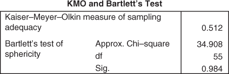
Table 4.8 provides the results of these statistical tests. The KMO statistic has a value of 0.549, which is not less than 0.5, meaning that this test does not find the level of correlation to be too low for factor analysis. The p-value for Bartlett's Test of Sphericity rounds to zero, so that the null hypothesis that no correlation exists among the variables is rejected. We therefore proceed with the factor analysis.
Table 4.8 Is there sufficiently high correlation to run factor analysis?
| KMO and Bartlett's Test | ||
| Kaiser–Meyer–Olkin measure of sampling adequacy | 0.549 | |
| Bartlett's test of sphericity | Approx. Chi-square | 1397.824 |
| df | 10 | |
| p-Value | 0.000 | |
To allow us to view the results using a scatter plot, we decide a priori to extract only two factors. The following factor analysis is performed using the principal axis factoring option. In principal axis factoring, an iterative procedure is used to estimate the communalities and the factor solution. This particular analysis required 152 such iterations before reaching convergence. The eigenvalues and the proportions of the variance explained by each factor are shown in Table 4.9.
Table 4.9 Eigenvalues and proportions of variance explained, factor analysis
| Total Variance Explained | |||
| Initial Eigenvalues | |||
| Factor | Total | % of Variance | Cumulative% |
| 1 | 1.277 | 25.533 | 25.533 |
| 2 | 1.036 | 20.715 | 46.248 |
| 3 | 0.951 | 19.028 | 65.276 |
| 4 | 0.912 | 18.241 | 83.517 |
| 5 | 0.824 | 16.483 | 100.000 |
Extraction method: Principal axis factoring.
Note that the first two factors extract less than half of the total variability in the variables, as contrasted with the houses data set, where the first two components extracted over 72% of the variability. This is due to the weaker correlation structure inherent in the original data.
The factor loadings ![]() are shown in Table 4.10. Factor loadings are analogous to the component weights in PCA, and represent the correlation between the ith variable and the jth factor. Notice that the factor loadings are much weaker than the previous houses example, again due to the weaker correlations among the standardized variables.
are shown in Table 4.10. Factor loadings are analogous to the component weights in PCA, and represent the correlation between the ith variable and the jth factor. Notice that the factor loadings are much weaker than the previous houses example, again due to the weaker correlations among the standardized variables.
Table 4.10 Factor loadings are much weaker than previous example
| Factor Matrixa | ||
| Factor | ||
| 1 | 2 | |
| AGE_Z | 0.590 | −0.329 |
| EDUC_Z | 0.295 | 0.424 |
| CAPNET_Z | 0.193 | 0.142 |
| HOURS_Z | 0.224 | 0.193 |
| DEM_Z | −0.115 | 0.013 |
Extraction method: Principal axis factoring.
a Two factors extracted. 152 iterations required.
The communalities are also much weaker than the houses example, as shown in Table 4.11. The low communality values reflect the fact that there is not much shared correlation among the variables. Note that the factor extraction increases the shared correlation.
Table 4.11 Communalities are low, reflecting not much shared correlation
| Communalities | ||
| Initial | Extraction | |
| AGE_Z | 0.015 | 0.457 |
| EDUC_Z | 0.034 | 0.267 |
| CAPNET_Z | 0.021 | 0.058 |
| HOURS_Z | 0.029 | 0.087 |
| DEM_Z | 0.008 | 0.013 |
Extraction method: Principal axis factoring.
4.10 Factor Rotation
To assist in the interpretation of the factors, factor rotation may be performed. Factor rotation corresponds to a transformation (usually orthogonal) of the coordinate axes, leading to a different set of factor loadings. We may look upon factor rotation as analogous to a scientist attempting to elicit greater contrast and detail by adjusting the focus of the microscope.
The sharpest focus occurs when each variable has high factor loadings on a single factor, with low-to-moderate loadings on the other factors. For the houses example, this sharp focus occurred already on the unrotated factor loadings (e.g., Table 4.5), so rotation was not necessary. However, Table 4.10 shows that we should perhaps try factor rotation for the adult data set, in order to help improve our interpretation of the two factors.
Figure 4.6 shows the graphical view of the vectors of factors of loadings for each variable from Table 4.10. Note that most vectors do not closely follow the coordinate axes, which means that there is poor “contrast” among the variables for each factor, thereby reducing interpretability.

Figure 4.6 Unrotated vectors of factor loadings do not follow coordinate axes.
Next, a varimax rotation (discussed shortly) was applied to the matrix of factor loadings, resulting in the new set of factor loadings found in Table 4.12. Note that the contrast has been increased for most variables, which is perhaps made clearer by Figure 4.7, the graphical view of the rotated vectors of factor loadings.
Table 4.12 The factor loadings after varimax rotation
| Rotated Factor Matrixa | ||
| Factor | ||
| 1 | 2 | |
| AGE_Z | 0.675 | 0.041 |
| EDUC_Z | 0.020 | 0.516 |
| CAPNET_Z | 0.086 | 0.224 |
| HOURS_Z | 0.084 | 0.283 |
| DEM_Z | −0.104 | −0.051 |
Extraction method: Principal axis factoring.
Rotation method: Varimax with Kaiser normalization.
a Rotation converged in three iterations.
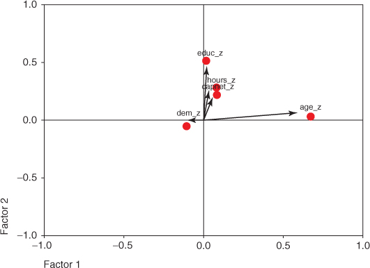
Figure 4.7 Rotated vectors of factor loadings more closely follow coordinate axes.
Figure 4.7 shows that the factor loadings have been rotated along the axes of maximum variability, represented by Factor 1 and Factor 2. Often, the first factor extracted represents a “general factor,” and accounts for much of the total variability. The effect of factor rotation is to redistribute this first factor's variability explained among the second, third, and subsequent factors. For example, consider Table 4.13, which shows the percent of variance explained by Factors 1 and 2, for the initial unrotated extraction (left side) and the rotated version (right side).
Table 4.13 Factor rotation redistributes the percentage of variance explained
| Total Variance Explained | ||||||
| Extraction Sums of Squared Loadings | Rotation Sums of Squared Loadings | |||||
| Factor | Total | % of Variance | Cumulative% | Total | % of Variance | Cumulative% |
| 1 | 0.536 | 10.722 | 10.722 | 0.481 | 9.616 | 9.616 |
| 2 | 0.346 | 6.912 | 17.635 | 0.401 | 8.019 | 17.635 |
Extraction method: Principal axis factoring.
The sums of squared loadings for Factor 1 for the unrotated case is (using Table 4.10 and allowing for rounding, as always) ![]() .
.
This represents 10.7% of the total variability, and about 61% of the variance explained by the first two factors. For the rotated case, Factor 1's influence has been partially redistributed to Factor 2 in this simplified example, now accounting for 9.6% of the total variability and about 55% of the variance explained by the first two factors.
We now describe three methods for orthogonal rotation, in which the axes are rigidly maintained at 90°. The goal when rotating the matrix of factor loadings is to ease interpretability by simplifying the rows and columns of the column matrix. In the following discussion, we assume that the columns in a matrix of factor loadings represent the factors, and that the rows represent the variables, just as in Table 4.10, for example. Simplifying the rows of this matrix would entail maximizing the loading of a particular variable on one particular factor, and keeping the loadings for this variable on the other factors as low as possible (ideal: row of zeroes and ones). Similarly, simplifying the columns of this matrix would entail maximizing the loading of a particular factor on one particular variable, and keeping the loadings for this factor on the other variables as low as possible (ideal: column of zeroes and ones).
- Quartimax Rotation seeks to simplify the rows of a matrix of factor loadings. Quartimax rotation tends to rotate the axes so that the variables have high loadings for the first factor, and low loadings thereafter. The difficulty is that it can generate a strong “general” first factor, in which many variables have high loadings.
- Varimax Rotation prefers to simplify the column of the factor loading matrix. Varimax rotation maximizes the variability in the loadings for the factors, with a goal of working toward the ideal column of zeroes and ones for each variable. The rationale for varimax rotation is that we can best interpret the factors when they are strongly associated with some variable and strongly not associated with other variables. Kaiser10 showed that the varimax rotation is more invariant than the quartimax rotation.
- Equimax Rotation seeks to compromise between simplifying the columns and the rows.
The researcher may prefer to avoid the requirement that the rotated factors remain orthogonal (independent). In this case, oblique rotation methods are available, in which the factors may be correlated with each other. This rotation method is called oblique because the axes are no longer required to be at 90°, but may form an oblique angle. For more on oblique rotation methods, see Harmon.11
4.11 User-Defined Composites
Factor analysis continues to be controversial, in part due to the lack of invariance under transformation, and the consequent nonuniqueness of the factor solutions. Analysts may prefer a much more straightforward alternative: User-Defined Composites. A user-defined composite is simply a linear combination of the variables, which combines several variables together into a single composite measure. In the behavior science literature, user-defined composites are known as summated scales (e.g., Robinson et al., 1991).12
User-defined composites take the form ![]() , where
, where ![]() ,
, ![]() , and the
, and the ![]() are the standardized variables. Whichever form the linear combination takes, however, the variables should be standardized first, so that one variable with high dispersion does not overwhelm the others.
are the standardized variables. Whichever form the linear combination takes, however, the variables should be standardized first, so that one variable with high dispersion does not overwhelm the others.
The simplest user-defined composite is simply the mean of the variables. In this case, ![]() . However, if the analyst has prior information or expert knowledge available to indicate that the variables should not be all equally weighted, then each coefficient
. However, if the analyst has prior information or expert knowledge available to indicate that the variables should not be all equally weighted, then each coefficient ![]() can be chosen to reflect the relative weight of that variable, with more important variables receiving higher weights.
can be chosen to reflect the relative weight of that variable, with more important variables receiving higher weights.
What are the benefits of utilizing user-defined composites? When compared to the use of individual variables, user-defined composites provide a way to diminish the effect of measurement error. Measurement error refers to the disparity between the observed variable values, and the “true” variable value. Such disparity can be due to a variety of reasons, including mistranscription and instrument failure. Measurement error contributes to the background error noise, interfering with the ability of models to accurately process the signal provided by the data, with the result that truly significant relationships may be missed. User-defined composites reduce measurement error by combining multiple variables into a single measure.
Appropriately constructed user-defined composites allow the analyst to represent the manifold aspects of a particular concept using a single measure. Thus, user-defined composites enable the analyst to embrace the range of model characteristics, while retaining the benefits of a parsimonious model.
Analysts should ensure that the conceptual definition for their user-defined composites lies grounded in prior research or established practice. The conceptual definition of a composite refers to the theoretical foundations for the composite. For example, have other researchers used the same composite, or does this composite follow from best practices in one's field of business? If the analyst is aware of no such precedent for his or her user-defined composite, then a solid rationale should be provided to support the conceptual definition of the composite.
The variables comprising the user-defined composite should be highly correlated with each other and uncorrelated with other variables used in the analysis. This unidimensionality should be confirmed empirically, perhaps through the use of PCA, with the variables having high loadings on a single component and low-to-moderate loadings on the other components.
4.12 An Example of a User-Defined Composite
Consider again the houses data set. Suppose that the analyst had reason to believe that the four variables, total rooms, total bedrooms, population, and households, were highly correlated with each other and not with other variables. The analyst could then construct the following user-defined composite:
with ![]() , so that Composite W represented the mean of the four (standardized) variables.
, so that Composite W represented the mean of the four (standardized) variables.
The conceptual definition of Composite W is “block group size,” a natural and straightforward concept. It is unlikely that all block groups have exactly the same size, and that therefore, differences in block group size may account for part of the variability in the other variables. We might expect large block groups tending to have large values for all four variables, and small block groups tending to have small values for all four variables.
The analyst should seek out support in the research or business literature for the conceptual definition of the composite. The evidence for the existence and relevance of the user-defined composite should be clear and convincing. For example, for Composite W, the analyst may cite the study from the National Academy of Sciences by Hope et al. (2003),13 which states that block groups in urban areas average 5.3 km2 in size while block groups outside urban areas averaged 168 km2 in size. As we may not presume that block groups inside and outside urban areas have exactly similar characteristics, this may mean that block group size could conceivably be associated with differences in block group characteristics, including median housing value, the response variable. Further, the analyst could cite the U.S. Census Bureau's notice in the Federal Register (2002)14 that population density was much lower for block groups whose size was greater than 2 square miles. Hence, block group size may be considered a “real” and relevant concept to be used in further analysis downstream.
R References
- Bernaards CA, Jennrich RI. 2005. Gradient projection algorithms and software for arbitraryrotation criteria in factor analysis, Educational and Psychological Measurement: 65, 676-696. http://www.stat.ucla.edu/research/gpa.
- R Core Team. R: A Language and Environment for Statistical Computing. Vienna, Austria: R Foundation for Statistical Computing; 2012. ISBN: 3-900051-07-0http://www.R-project.org/.
- Revelle W. 2013. psych: Procedures for Personality and Psychological Research, Northwestern University, Evanston, Illinois, USA, http://CRAN.R-project.org/package=psychVersion=1.4.2.
Exercises
Clarifying The Concepts
1. Determine whether the following statements are true or false. If false, explain why the statement is false, and how one could alter the statement to make it true.
- Positive correlation indicates that, as one variable increases, the other variable increases as well.
- Changing the scale of measurement for the covariance matrix, for example, from meters to kilometers, will change the value of the covariance.
- The total variability in the data set equals the number of records.
- The value of the ith principal component equals the ith eigenvalue divided by the number of variables.
- The second principal component represents any linear combination of the variables that accounts for the most variability in the data, once the first principal component has been extracted.
- For a component weight to be considered of practical significance, it should exceed
 in magnitude.
 - The principal components are always mutually exclusive and exhaustive of the variables.
- When validating the principal components, we would expect the component weights from the training and test data sets to have the same signs.
- For factor analysis to function properly, the predictor variables should not be highly correlated.
2. For what type of data are the covariance and correlation matrices identical? In this case, what is ![]() ?
?
3. What is special about the first principal component, in terms of variability?
4. Describe the four criteria for choosing how many components to extract. Explain the rationale for each.
5. Explain the concept of communality, so that someone new to the field could understand it.
6. Explain the difference between PCA and factor analysis. What is a drawback of factor analysis?
7. Describe two tests for determining whether there exists sufficient correlation within a data set for factor analysis to proceed. Which results from these tests would allow us to proceed?
8. Explain why we perform factor rotation. Describe three different methods for factor rotation.
9. What is a user-define composite, and what is the benefit of using it in place of individual variables?
Working With The Data
The following computer output explores the application of PCA to the Churn data set.
10. Based on the following information, does there exists an adequate amount of correlation among the predictors to pursue PCA? Explain how you know this, and how we may be getting mixed signals.15
11. Suppose that we go ahead and perform the PCA, in this case using seven components. Considering the following information, which variable or variables might we be well advised to omit from the PCA, and why? If we really need all these variables in the analysis, then what should we do?

12. Based on the following information, how many components should be extracted, using (a) the eigenvalue criterion and (b) the proportion of variance explained criterion?

13. Based on the following scree plot, how many components should be extracted using the scree plot criterion? Now, based on the three criteria, work toward a decision on the number of components to extract.

14. Based on the following rotated component matrix:
- Provide a quick profile of the first four components.
- If we extracted an eighth component, describe how the first component would change.
- What is your considered opinion on the usefulness of applying PCA on this data set?
Hands-On Analysis
For Exercises 15–20, work with the baseball data set, available from the textbook web site, www.DataMiningConsultant.com.
15. First, filter out all batters with fewer than 100 at bats. Next, standardize all the numerical variables using z-scores.
16. Now, suppose we are interested in estimating the number of home runs, based on the other numerical variables in the data set. So all the other numeric variables will be our predictors. Investigate whether sufficient variability exists among the predictors to perform PCA.
17. How many components should be extracted according to
- The Eigenvalue Criterion?
- The Proportion of Variance Explained Criterion?
- The Scree Plot Criterion?
- The Communality Criterion?
18. Based on the information from the previous exercise, make a decision about how many components you shall extract.
19. Apply PCA using varimax rotation, with your chosen number of components. Write up a short profile of the first few components extracted.
20. Construct a useful user-defined composite using the predictors. Describe situations where the composite would be more appropriate or useful than the principal components, and vice versa.
Use the wine_quality_training data set, available at the textbook web site, for the remaining exercises. The data consist of chemical data about some wines from Portugal. The target variable is quality. Remember to omit the target variable from the dimension-reduction analysis. Unless otherwise indicated, use only the white wines for the analysis.
21. Standardize the predictors.
22. Construct a matrix plot of the predictors. Provide a table showing the correlation coefficients of each predictor with each other predictor. Color code your table so that the reader can easily see at a glance which are the strongest correlations. What you are doing here is doing EDA for the principal components later on. Using the matrix plot and the table of coefficients, discuss which sets of predictors seem to “vary together.”
23. Suppose we eventually would like to perform linear regression analysis of quality versus these predictors. Clearly explain why we should beware of using a set of predictors that are highly correlated.
24. Run a multiple regression of the predictors on quality. Get the variance inflation factor (VIF) measures of the predictors. Explain what these mean in the context of this problem. Explain whether they support or undermine the need for PCA in this problem.
25. Clearly explain how PCA can solve the problem of collinear predictors.
26. Determine the optimal number of components to extract, using
- The Eigenvalue Criterion;
- The Proportion of Variance Explained Criterion;
- The Minimum Communality Criterion;
- The Scree Plot Criterion;
- Try to arrive at a consensus among the four criteria as to the optimal number of components to extract.
27. Proceed to apply PCA to the predictors, using varimax rotation. In the output, suppress factor loadings less than ![]() .
.
- Provide both the unrotated and the rotated component matrices.
- Use the results in (a) to demonstrate how varimax rotation eases interpretability of the components.
- Report detailed profiles of the components, including a descriptive title. It is important that you be able to explain to your client with crystal clarity what your results mean. It may be worth your while to do some research on wine.
28. Compare your principal components in one-to-one manner with your EDA earlier. Discuss.
29. Run a multiple regression of the principal components predictors on quality.
- Get the VIF measures of the components. Comment.
- Compare the regression standard error for the two regression models. Comment.
- Compare the
 for the two regression models. Comment.
30. Provide a table showing the correlation coefficients of each principal component with each other principal component. Comment.
31. Discuss the question of whether we should add principal components to increase the predictive power of the regression model and/or reduce the standard error. Arm yourself for this discussion by incrementing your optimal number of components by 1, running the PCA, performing the regression with the additional component, and then comparing your standard error and ![]() to the earlier model.
to the earlier model.
32. Repeat Exercises 21–31 using the red wines only. Compare your principal component profiles and the performance of your regression models.