
Chapter 17
Cost-Benefit Analysis for Trinary and -Nary Classification Models
Not all classification problems involve binary targets. For example, color researchers may be interested in user classification of colors such as red, blue, yellow, green, and so on. In earlier chapters, we dealt with cost-benefit analysis for classification models having a binary target variable only. In this chapter, we extend our analytic framework to encompass classification evaluation measures and data-driven misclassification costs, first for trinary targets, and then for k-nary targets in general.
17.1 Classification Evaluation Measures for a Generic Trinary Target
For the classification problem with a generic trinary target variable taking values A, B, and C, there are nine possible combinations of predicted/actual categories, as shown in Table 17.1. The contingency table for this generic trinary problem is as shown in Table 17.2.
Table 17.1 Definition and notation for the nine possible decision combinations, generic trinary variable
| Decision | Predicted | Actual | |
| A | A | ||
| B | B | ||
| C | C | ||
| A | B | ||
| A | C | ||
| B | A | ||
| B | C | ||
| C | A | ||
| C | B |
Table 17.2 Contingency table for generic trinary problem
 |
![]() may be considered a true A, analogous to a true positive or true negative decision in the binary case. Similarly,
may be considered a true A, analogous to a true positive or true negative decision in the binary case. Similarly, ![]() and
and ![]() may be viewed as a true B and a true C, respectively. Note, however, that the true positive/false positive/true negative/false negative usage is no longer applicable here for this trinary target variable. Thus, we need to define new classification evaluation measures.
may be viewed as a true B and a true C, respectively. Note, however, that the true positive/false positive/true negative/false negative usage is no longer applicable here for this trinary target variable. Thus, we need to define new classification evaluation measures.
We denote the marginal totals as follows. Let the total number of records predicted to belong to category A be denoted as
Similarly, the number of records predicted to belong to category B is given as
and the number of records predicted to belong to category C is given as
Also, let the total number of records actually belonging to category A be denoted as
Similarly, the number of actual category B records is given as
and the number of actual category C records is given as
The grand total ![]() represents the sum of all the cells in the contingency table.
represents the sum of all the cells in the contingency table.
Next, we define classification evaluation measures for the trinary case, extending and amending the similar well-known binary classification evaluation measures. For the binary case, sensitivity and specificity are defined as follows:
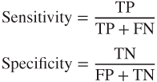
In the binary case, sensitivity is defined as the ratio of the number of true positives to the number of actual positives in the data set. Specificity is defined as the ratio of the number of true negatives to the number of actual negatives. For the trinary case, we analogously define the following measures:
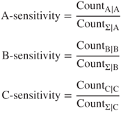
For example, A-sensitivity is the ratio of correctly predicted A-records to the total number of A-records. It is interpreted as the probability that a record is correctly classified as A, given that the record is actually belongs to the A class; similarly for B-sensitivity and C-sensitivity. No specificity measure is needed, because specificity in the binary case is essentially a type of sensitivity measure for the negative category.
Next, in the binary case, we have the following measures:

We extend these measures for the trinary case as follows:
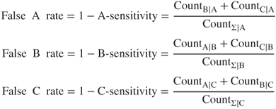
For example, the false A rate is interpreted as the ratio of incorrectly classified A-records to the total number of A-records. For the binary case, the proportion of true positives and the proportion of true negatives are given as follows:
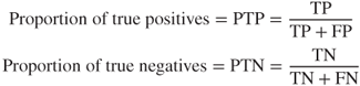
In the binary case, PTP is interpreted as the likelihood that the record is actually positive, given that it is classified as positive. Similarly, PTN is interpreted as the likelihood that the record is actually negative, given that it is classified as negative. For the trinary case, we have the following evaluation measures, analogously defined from the binary case:
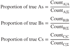
For example, the interpretation of the proportion of true As is the likelihood that a particular record actually belongs to class A, given that it is classified as A. Next we turn to the proportions of false positives and negatives, defined in the binary case as

We extend these measures for the trinary case as follows:
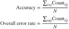
Finally, we have accuracy and the overall error rate, defined as follows:

17.2 Application of Evaluation Measures for Trinary Classification to the Loan Approval Problem
For the trinary target variable approval, there are nine combinations of predicted/actual categories as shown in Table 17.3.
Table 17.3 Definition and notation for the nine possible loan decision combinations
| Decision | Predicted | Actual | |
| Denied | Denied | ||
| Approved half | Approved half | ||
| Approved whole | Approved whole | ||
| Denied | Approved half | ||
| Denied | Approved whole | ||
| Approved half | Denied | ||
| Approved half | Approved whole | ||
| Approved whole | Denied | ||
| Approved whole | Approved half |
Table 17.4 presents the contingency table for a classification and regression trees (CART) model without misclassification costs applied to the Loans3_training data set and evaluated on the Loans3_test data set. Note that the Loans3 data sets are similar to the Loans data sets except for record distribution between the two data sets, and the change from a binary target to a trinary target. We denote the marginal totals as follows. Let the total number of records predicted to be denied as
Table 17.4 Contingency table of CART model without misclassification costs (“model 1”), evaluated on Loans3_test data set
 |
Similarly, let the number of customers predicted to be approved for funding at half the requested loan amount as
and let the number of customers predicted to be approved for funding at the whole requested loan amount as
Also, let the total number of customers who are actually financially insecure and should have been denied a loan as
Similarly, the number of customers who are actually somewhat financially secure and should have been approved for a loan at half the requested amount as
and let the number of customers who are actually quite financially secure and should have been approved for a loan at the whole requested amount as
Let the grand total ![]() represent the sum of all the cells in the contingency table.
represent the sum of all the cells in the contingency table.
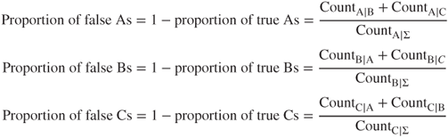
We are interested in evaluating our contingency tables using the trinary classification evaluation measures developed earlier. These are adapted to the trinary loan classification problem as follows:
For example, D-sensitivity is the ratio of the number of applicants correctly denied a loan to the total number of applicants who were denied a loan. This is interpreted as the probability that an applicant is correctly classified as Denied, given that the applicant actually belongs to the denied class. The CART model is less sensitive to the presence of approved half applicants than the other classes. For example, AH-sensitivity = 0.81 indicates that the ratio of the number of applicants correctly denied a loan to the total number of applicants who were denied a loan. In other words, the probability is 0.81 that an applicant is correctly classified as approved half, given that the applicant actually belongs to the approved half class.
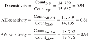
Next, we have the following:

For example, as the complement of D-sensitivity, the false D rate is interpreted as the probability that an applicant is not classified as denied, even though the applicant actually belongs to the denied class. In this case, this probability is 0.06. Note that the false AH rate is three times that of the other rates, indicating that we can be less confident in the classifications our model makes of the approved half category.
For the three classes, the proportions of true classifications are specified as follows:

For example, if a particular applicant is classified as denied, then the probability that this customer actually belongs to the denied class is 0.93. This is higher than the analogous measures for the other classes, especially AH.
Next, we find the additive inverses of these measures as follows:
For instance, if an applicant is classified as approved half, there is a 15% chance that the applicant actually belongs to a different class.
Finally, the accuracy is given as follows:
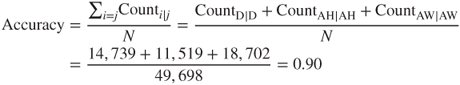
and the overall error rate is as follows:

That is, across all classes, our model classifies 90% of the applicants correctly, and misclassifies only 10% of all applicants.
17.3 Data-Driven Cost-Benefit Analysis for Trinary Loan Classification Problem
To conduct a data-driven cost-benefit analysis, we look to the data to tell us what the costs and benefits of the various decisions will be.
- Principal. Using the Loans3_training data set, we find that the mean amount requested is $13,427.
- Thus, for loans approved for the entire amount, the loan principal will be modeled as $13,427.
- For loans approved for only half the amount, the loan principal will be set as half of $13,427, which is $6713.50.
- Interest. From the Loans3_training data set, the mean amount of loan interest is $6042.
- Thus, for loans approved for the whole amount, the loan interest is set to $6042.
- For loans approved for only half the amount, the loan interest is modeled as half of $6042; that is, $3021.
- Simplifying Assumptions. For simplicity, we make the following assumptions:
- The only costs and gains that we model are principal and interest. Other types of costs such as clerical costs are ignored.
- If a customer defaults on a loan, the default is assumed to occur essentially immediately, so that no interest is accrued to the bank from such loans.
On the basis of these data-driven specifications and simplifying assumptions, we proceed to calculate the costs as follows.
 : Correctly predict that an applicant should be denied. This represents an applicant who would not have been able to repay the loan (i.e., defaulted) being correctly classified for non-approval. The direct cost incurred for this applicant is zero. As no loan was proffered, there could be neither interest incurred nor any default made. Thus, the cost is $0.
 : Predict loan approval at half the requested amount, when the applicant should have been denied the loan. The customer will default immediately, so that the bank receives no interest. Plus the bank will lose the entire amount loaned, which equals on average $6713.50, or half the average requested amount in the data set. Thus, the cost for this error is $6713.50.
 : Predict loan approval at the whole requested amount, when the applicant should have been denied the loan. This is the most expensive error the bank can make. On average, the bank will lose $13,427, or the average loan request amount, for each of these errors, so the cost is $13,427.
 : Predict loan denial when the applicant should have been approved for half the requested loan amount. As no loan was proffered, there could be neither interest incurred nor any default made. Thus, the cost is $0.
 : Correctly predict than an applicant should be approved for funding half of the requested loan amount. This represents an applicant who would reliably repay the loan at half the requested amount being correctly classified for loan approval at this level. The bank stands to make $3021 (half the mean amount of loan interest) from customers such as this. So the cost for this applicant −$3021.
 : Predict loan approval at the whole requested amount, when the applicant should have been approved at only half the requested amount. The assumption is that the applicant will pay off half the loan, the bank will receive the interest for half of the loan (cost = −$3021), and then the applicant will immediately default for the remainder of the loan (cost = $6713.50). Thus, the cost of this error is $3692.50 ($6713.50 − $3021).
 : Predict loan denial when the applicant should have been approved for the whole loan amount. Again, no loan was proffered, so the cost is $0.
 : Predict loan approval at half the requested amount, when the applicant should have been approved for the entire requested loan amount. This financially secure customer will presumably be able to pay off this smaller loan, so that the bank will earn $3021 (half the mean amount of loan interest from the data set). Thus, the cost is −$3021.
 : Correctly predict than an applicant should be approved for funding the whole requested loan amount. This represents an applicant who would reliably repay the entire loan being correctly classified for loan approval at this level. The bank stands to make $6042 (the mean amount of loan interest) from customers such as this. So the cost for this applicant −$6042.
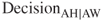
We assemble these costs into the cost matrix shown in Table 17.5.
Table 17.5 Cost matrix for the trinary loan classification problem. Use this matrix form for calculating the total cost of the model
 |
17.4 Comparing Cart Models With and Without Data-Driven Misclassification Costs
Let us see what the effects are of using the data-driven misclassification costs for our CART model. We would like the diagonal elements of the total cost matrix to contain zeroes, because software such as IBM SPSS Modeler requires such a structure when setting the misclassification costs. By decision invariance under cost matrix row adjustment (Chapter 16), a classification decision is not changed by the addition or subtraction of a constant from the cells in the same row of a cost matrix. Thus, we can obtain our desired cost matrix with zeroes on the diagonal by
- not altering the first row;
- adding $3021 to each cell in the second row;
- adding $6042 to each cell in the third row.
We then obtain the direct cost matrix with zeroes on the diagonal as shown in Table 17.6. For simplicity and perspective, the costs in Table 17.6 were scaled by the minimum nonzero entry $3021, giving us the scaled cost matrix in Table 17.7. The scaled costs in Table 17.7 were then used as the software misclassification costs to construct a CART model for predicting loan approval, based on the Loans3_training data set. The resulting contingency table obtained by evaluating this model with the Loans3_test data set is provided in Table 17.8.
Table 17.6 Cost matrix with zeroes on the diagonal
 |
Table 17.7 Scaled cost matrix
 |
Table 17.8 Contingency table of CART model with misclassification costs (“model 2”)
 |
Table 17.9 contains a comparison of the classification evaluation measures we have examined in this chapter for the two models. (Calculations for the model with misclassification costs are not shown, to save space.) Denote the model without misclassification costs as model 1 and the model with misclassification costs as model 2. Note that the measures within a cell sum to 1, indicating that the measures are additive inverses. For each metric, the better performing model is indicated in bold.
Table 17.9 Comparison of evaluation measures for CART models with and without misclassification costs (better performance highlighted)
| Evaluation Measure | CART Model | |
| Model 1: Without | Model 2: With | |
| Misclassification Costs | Misclassification Costs | |
| D-sensitivity | 0.94 | 0.94 |
| False D rate | 0.06 | 0.06 |
| AH-sensitivity | 0.81 | 0.89 |
| False AH rate | 0.19 | 0.11 |
| AW-sensitivity | 0.94 | 0.85 |
| False AW rate | 0.06 | 0.15 |
| Proportion of true Ds | 0.93 | 0.93 |
| Proportion of false Ds | 0.07 | 0.07 |
| Proportion of true AHs | 0.85 | 0.77 |
| Proportion of false AHs | 0.15 | 0.23 |
| Proportion of true AWs | 0.92 | 0.98 |
| Proportion of false AWs | 0.08 | 0.02 |
| Accuracy | 0.90 | 0.89 |
| Overall error rate | 0.10 | 0.11 |
We may observe the following points of interest from the comparison provided in Table 17.9.
- Interestingly, the counts in the leftmost column of the contingency table for both models are the same, indicating that there is no difference in the models with respect to predicting the denied category. This is supported by the exact same values for proportion of true Ds and proportion of false Ds. (The values for D-sensitivity and false D rate are similar, but not exactly the same, apart from rounding.)
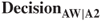
- The AH-sensitivity of model 2 is superior, because it makes fewer errors of the form
 . This is presumably because of the misclassification cost associated with this decision.
 - The AW-sensitivity of model 1 is superior, because it makes fewer errors of the form
 . One may speculate that this is because the generally high misclassification costs associated with classifying an applicant as approved whole have tended to make our model shy about making such a classification, thereby pushing some
  decisions into the
  cell.
cell. - The proportion of true AHs of model 1 is superior, again because it makes fewer errors of the form
 , and perhaps for the same reason as mentioned above.
 - The proportion of true AWs of model 2 is superior, because model 2 makes fewer errors of the form
 and of the form
  .
. - The accuracy and overall error rate of model 1 is slightly better. Does this mean that model 1 is superior overall?
When the business or research problem calls for misclassification costs, then the best metric for comparing the performance of two or models is overall cost of the model. Using the cost matrix from Table 17.5, we find the overall cost of model 1 (from Table 17.4) to be ![]() , for a per-applicant profit of $2800.19. The overall cost for model 1 (from Table 17.8) is
, for a per-applicant profit of $2800.19. The overall cost for model 1 (from Table 17.8) is ![]() , with a profit of $2839.92 per applicant.
, with a profit of $2839.92 per applicant.
Thus, the estimated revenue increase from using model 2 rather than model 1 is given as follows:
Thus, model 2 is superior, in the way that counts the most, on the bottom line. In fact, simply by applying data-driven misclassification costs to our CART model, we have enhanced our estimated revenue by nearly $2 million. Now, that should be enough to earn the hardworking data analyst a nice holiday bonus.
17.5 Classification Evaluation Measures for a Generic k-Nary Target
For the classification problem with a generic k-nary target variable taking values ![]() , there are
, there are ![]() possible combinations of predicted/actual categories, as shown in Table 17.10.
possible combinations of predicted/actual categories, as shown in Table 17.10.
Table 17.10 The k2 possible decision combinations, generic k-nary variable
| Decision | Predicted | Actual | |
The contingency table for this generic k-nary problem is shown in Table 17.11.
Table 17.11 Contingency table for generic k-nary problem
 |
The marginal totals are defined analogously to the trinary case, and again we let the grand total ![]() represent the sum of all the cells in the contingency table.
represent the sum of all the cells in the contingency table.
Next, we define classification evaluation measures for the k-nary case, extending the trinary case. For the ith class, we define sensitivity as follows:
Here ![]() is the ratio of correctly predicted
is the ratio of correctly predicted ![]() -records to the total number of
-records to the total number of ![]() -records. It is interpreted as the probability that a record is correctly classified
-records. It is interpreted as the probability that a record is correctly classified ![]() , given that the record actually belongs to the
, given that the record actually belongs to the ![]() class. Next, the false
class. Next, the false ![]() rate is given by the following equation:
rate is given by the following equation:

The false ![]() rate is interpreted as the ratio of incorrectly classified
rate is interpreted as the ratio of incorrectly classified ![]() -records to the total number of
-records to the total number of ![]() -records. Next, we have
-records. Next, we have
and

Finally, the accuracy and the overall error rate are defined as
17.6 Example of Evaluation Measures and Data-Driven Misclassification Costs for k-Nary Classification
The Loans4_training and Loans4_test data sets are used to illustrate classification evaluation measures for a target with four classes. Note that the Loans4 data sets are similar to the Loans data sets except for record distribution between the two data sets, and the change from a binary target to a quaternary (k-nary with k = 4) target. In this case, the target classes are denied, approved 1/3, approved 2/3, and approved whole. Approved 1/3 (denoted as A1 below) indicates that the applicant was approved for only one-third of the loan request amount, and Approved 2/3 (denoted A2) indicates approval of two-thirds of the request amount. A CART model was trained on the Loans4_training data set without misclassification costs, and fit to the data in the Loans4_test data set, with the resulting contingency table provided in Table 17.12.
Table 17.12 Contingency table of CART model without misclassification costs, for the Loans4 target with four classes
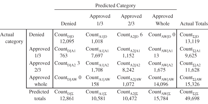 |
Again, to conduct a data-driven cost-benefit analysis, we look to the data to tell us what the costs and benefits of the various decisions will be. The mean amount of the principal for the training set is still $13,427, so that loans approved for only one-third or two-thirds of the full amount will have principal set as ![]() and
and ![]() , respectively. The mean amount of interest for the training set is still $6042, so that loans approved for only one-third or two-thirds of the whole amount will have interest set as
, respectively. The mean amount of interest for the training set is still $6042, so that loans approved for only one-third or two-thirds of the whole amount will have interest set as ![]() and
and ![]() , respectively. The assumptions are the same as for the trinary case.
, respectively. The assumptions are the same as for the trinary case.
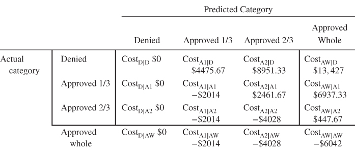
The cost matrix for this quaternary classification framework is given in Table 17.13. The reader is asked to justify these costs in the exercises. Here is a sample justification for the direct costs for ![]() .
.
 : Predict loan approval at the whole requested amount, when the applicant should have been approved at only two-thirds the requested amount. The assumption is that the applicant will pay off two-thirds of the loan, the bank will receive the interest for two-thirds of the loan (Cost = −$4028), and then the applicant will immediately default for the remainder of the loan (Cost = $4475.67). Thus, the cost of this error is $447.67 ($4475.67 − $4028).
Table 17.13 Cost matrix for quaternary classification framework
 |
In the exercises, the reader is asked to adjust the cost matrix into a form amenable to software analysis.
Misclassification costs supplied by the adjusted cost matrix from Table 17.13 (and constructed in the exercises) were applied to a CART model, with the resulting contingency table shown in Table 17.14.
Table 17.14 Contingency table of CART model with misclassification costs, for the Loans4 target with four classes
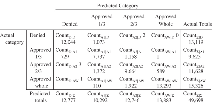 |
Table 17.15 contains a comparison of the classification evaluation measures for the models with and without misclassification costs. Denote the model without misclassification costs as model 3 and the model with misclassification costs as model 4. For each metric, the better performing model is indicated in bold. The evaluation metrics are mixed, with some metrics favoring each model. However, for the most important metric, that of total model cost, model 4 is superior.
Table 17.15 Comparison of evaluation measures for quaternary CART models with and without misclassification costs (better performance highlighted)
| Evaluation Measure | CART Model | |
| Model 3: Without | Model 4: With | |
| Misclassification | Misclassification | |
| Costs | Costs | |
| D-sensitivity | 0.92 | 0.91 |
| False D rate | 0.08 | 0.09 |
| A1-sensitivity | 0.80 | 0.84 |
| False A1 rate | 0.20 | 0.16 |
| A2-sensitivity | 0.83 | 0.77 |
| False AW rate | 0.17 | 0.23 |
| AW-sensitivity | 0.87 | 0.92 |
| False AW rate | 0.13 | 0.08 |
| Proportion of true Ds | 0.94 | 0.96 |
| Proportion of false Ds | 0.06 | 0.04 |
| Proportion of true A1s | 0.75 | 0.74 |
| Proportion of false A1s | 0.25 | 0.26 |
| Proportion of true A2s | 0.76 | 0.81 |
| Proportion of false A2s | 0.24 | 0.19 |
| Proportion of true AW's | 0.96 | 0.92 |
| Proportion of false AWs | 0.04 | 0.08 |
| Accuracy | 0.86 | 0.87 |
| Overall error rate | 0.14 | 0.13 |
The overall cost of model 3 is ![]() , with a per-applicant cost of
, with a per-applicant cost of ![]() , while the overall cost of model 4 is
, while the overall cost of model 4 is ![]() , with a per-applicant cost of
, with a per-applicant cost of ![]() . The increase in revenue per applicant from using misclassification costs is $80, with a total revenue increase of
. The increase in revenue per applicant from using misclassification costs is $80, with a total revenue increase of
Thus, the model constructed using data-driven misclassification costs increases the bank's revenue by nearly $4 million. However, the trinary models (models 1 and 2) outperformed the quaternary models (models 3 and 4) in terms of overall cost.
R References
- Therneau T, Atkinson B, Ripley B. 2013. rpart: Recursive partitioning. R package version 4.1-3. http://CRAN.R-project.org/package=rpart.
- R Core Team. R: A Language and Environment for Statistical Computing. Vienna, Austria: R Foundation for Statistical Computing; 2012. ISBN: 3-900051-07-0, http://www.R-project.org/.
Exercises
Clarifying The Concepts
1. Explain why the true positive/false positive/true negative/false negative usage is not applicable to classification models with trinary targets.
2. Explain the ![]() notation used in the notation in this chapter, for the marginal totals and the grand total of the contingency tables.
notation used in the notation in this chapter, for the marginal totals and the grand total of the contingency tables.
3. Explain why we do not use a specificity measure for a trinary classification problem.
4. What is the relationship between false A rate and A-sensitivity?
5. How are A-sensitivity and false A rate interpreted?
6. Why do we avoid the term positive predictive value in this book?
7. What is the relationship between the proportion of true As and the proportion of false As?
8. Interpret the proportion of true As and the proportion of false As.
9. Use the term “diagonal elements of the contingency table” to define (i) accuracy and (ii) overall error rate.
10. Express in your own words how we interpret the following measures:
- D-sensitivity, where D represents the denied class in the Loans problem
- False D rate
- Proportion of true Ds
- Proportion of false Ds.
11. Explain how we determine the principal and interest amounts for the Loans problem.
12. Why do we adjust our cost matrix so that there are zeroes on the diagonal?
13. Which cost matrix should we use when comparing models?
14. When misclassification costs are involved, what is the best metric for comparing model performance?
Working With The Data
15. Provide justifications for each of the direct costs given in Table 17.5.
16. Adjust Table 17.13 so that there are zeroes on the diagonal and the matrix is scaled, similarly to Table 17.7.
17. Using the results in Tables 17.12 and 17.14, confirm the values for the evaluation measures in Table 17.15.
Hands-On Analysis
18. On your own, recapitulate the trinary classification analysis undertaken in this chapter using the Loans3 data sets. (Note that the results may differ slightly due to different settings in the CART models.) Report all salient results, including a summary table, similarly to Table 17.9.
19. On your own, recapitulate the trinary classification analysis undertaken in this chapter using the Loans4 data sets. (Note that the results may differ slightly due to different settings in the CART models.) Report all salient results, including a summary table, similarly to Table 17.15.