Classification rule learning algorithms utilize a heuristic known as separate and conquer. The process involves identifying a rule that covers a subset of examples in the training data, and then separating this partition from the remaining data. As rules are added, additional subsets of data are separated until the entire dataset has been covered and no more examples remain.

One way to imagine the rule learning process is to think about drilling down into data by creating increasingly specific rules for identifying class values. Suppose you were tasked with creating rules for identifying whether or not an animal is a mammal. You could depict the set of all animals as a large space, as shown in the following diagram:

A rule learner begins by using the available features to find homogeneous groups. For example, using a feature that measured whether the species travels via land, sea, or air, the first rule might suggest that any land-based animals are mammals:

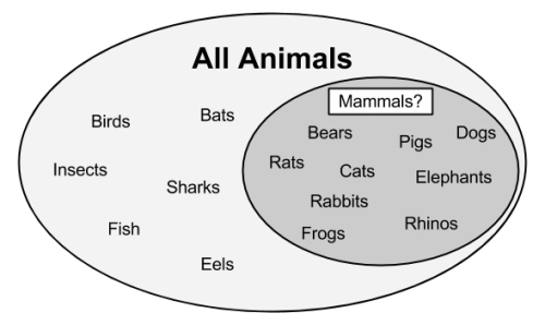
Do you notice any problems with this rule? If you look carefully, you might note that frogs are amphibians, not mammals. Therefore, our rule needs to be a bit more specific. Let's drill down further by suggesting that mammals walk on land and have a tail:

As shown in the previous figure, our more specific rule results in a subset of animals that are entirely mammals. Thus, this subset can be separated from the other data and additional rules can be defined to identify the remaining mammal bats. A potential feature distinguishing bats from the other remaining animals would be the presence of fur. Using a rule built around this feature, we have then correctly identified all the animals:

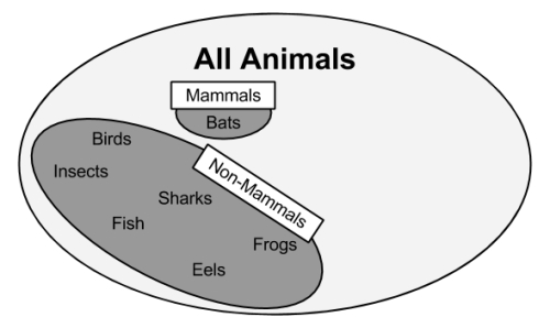
At this point, since all of the training instances have been classified, the rule learning process would stop. We learned a total of three rules:

The previous example illustrates how rules gradually consume larger and larger segments of data to eventually classify all instances. Divide-and-conquer and separate-and-conquer algorithms are known as greedy learners because data is used on a first-come, first-served basis.

As the rules seem to cover portions of the data, separate-and-conquer algorithms are also known as covering algorithms, and the rules are called covering rules. In the next section, we will learn how covering rules are applied in practice by examining a simple rule-learning algorithm. We will then examine a more complex rule learner, and apply both to a real-world problem.

Suppose that as part of a television game show, there was a wheel with ten evenly-sized colored slices. Three of the segments were colored red, three were blue, and four were white. Prior to spinning the wheel, you are asked to choose one of these colors. When the wheel stops spinning, if the color shown matches your prediction, you win a large cash prize. What color should you pick?

If you choose white, you are of course more likely to win the prize—this is the most common color on the wheel. Obviously, this game show is a bit ridiculous, but it demonstrates the simplest classifier, ZeroR, a rule learner that literally learns no rules (hence the name). For every unlabeled example, regardless of the values of its features, it predicts the most common class.

The One Rule algorithm (1R or OneR), improves over ZeroR by selecting a single rule. Although this may seem overly simplistic, it tends to perform better than you might expect. As Robert C. Holte showed in a 1993 paper, Very Simple Classification Rules Perform Well on Most Commonly Used Datasets (in Machine Learning, Vol. 11, pp. 63-91), the accuracy of this algorithm can approach that of much more sophisticated algorithms for many real-world tasks. The strengths and weaknesses of this algorithm are shown in the following table:

The way this algorithm works is simple. For each feature, 1R divides the data into groups based on similar values of the feature. Then, for each segment, the algorithm predicts the majority class. The error rate for the rule based on each feature is calculated, and the rule with the fewest errors is chosen as the one rule.

The following tables show how this would work for the animal data we looked at earlier in this section:

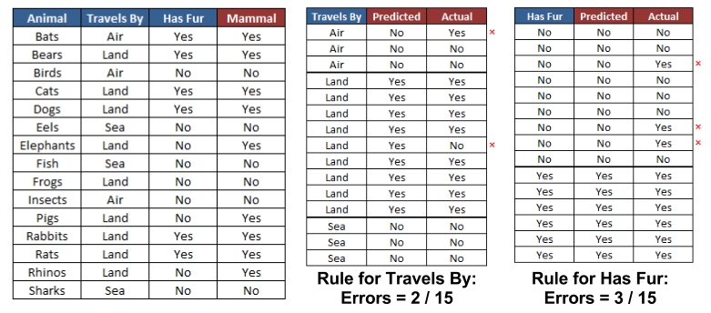
For the Travels By feature, the data was divided into three groups: Air, Land, and Sea. Animals in the Air and Sea groups were predicted to be non-mammal, while animals in the Land group were predicted to be mammals. This resulted in two errors: bats and frogs. The Has Fur feature divided animals into two groups. Those with fur were predicted to be mammals, while those without were not. Three errors were counted: pigs, elephants, and rhinos. As the Travels By feature resulted in fewer errors, the 1R algorithm would return the following "one rule" based on Travels By:

The algorithm stops here, having found the single most important rule.

Obviously, this rule learning algorithm may be too basic for some tasks. Would you want a medical diagnosis system to consider only a single symptom, or an automated driving system to stop or accelerate your car based on only a single factor? For these types of tasks a more sophisticated rule learner might be useful. We'll learn about one in the following section.

Early rule-learning algorithms were plagued by a couple of problems. First, they were notorious for being slow, making them ineffective for the increasing number of Big Data problems. Secondly, they were often prone to being inaccurate on noisy data.

A first step toward solving these problems was proposed in a 1994 paper by Johannes Furnkranz and Gerhard Widmer, Incremental Reduced Error Pruning (in Proceedings of the 11th International Conference on Machine Learning, pp. 70-77). The Incremental Reduced Error Pruning algorithm (IREP) uses a combination of pre-pruning and post-pruning methods that grow very complex rules and prune them before separating the instances from the full dataset. Although this strategy helped the performance of rule learners, decision trees often still performed better.

Rule learners took another step forward in 1995 with the publication of a landmark paper by William W. Cohen, Fast Effective Rule Induction (in Proceedings of the 12th International Conference on Machine Learning, pp. 115-123). This paper introduced the RIPPER algorithm (Repeated Incremental Pruning to Produce Error Reduction), which improved upon IREP to generate rules that match or exceed the performance of decision trees.

As outlined in the following table, the strengths and weaknesses of RIPPER rule learners are generally comparable to decision trees. The chief benefit is that they may result in a slightly more parsimonious model.

Having evolved from several iterations of rule-learning algorithms, the RIPPER algorithm is a patchwork of efficient heuristics for rule learning. Due to its complexity, a discussion of the technical implementation details is beyond the scope of this book. However, it can be understood in general terms as a three-step process:

The growing process uses separate-and-conquer technique to greedily add conditions to a rule until it perfectly classifies a subset of data or runs out of attributes for splitting. Similar to decision trees, the information gain criterion is used to identify the next splitting attribute. When increasing a rule's specificity no longer reduces entropy, the rule is immediately pruned. Steps one and two are repeated until reaching a stopping criterion, at which point the entire set of rules are optimized using a variety of heuristics.

The rules from RIPPER can be more complex than 1R, with multiple antecedents. This means that it can consider multiple attributes like "if an animal flies and has fur, then it is a mammal." This improves the algorithm's ability to model complex data, but just like decision trees, it means that the rules can quickly become more difficult to comprehend.

Classification rules can also be obtained directly from decision trees. Beginning at a leaf node and following the branches back to the root, you will have obtained a series of decisions. These can be combined into a single rule. The following figure shows how rules could be constructed from the decision tree for predicting movie success:

Following the paths from the root to each leaf, the rules would be:

The chief downside to using a decision tree to generate rules is that the resulting rules are often more complex than those learned by a rule-learning algorithm. The divide-and-conquer strategy employed by decision trees biases the results differently than that of a rule learner. On the other hand, it is sometimes more computationally efficient to generate rules from trees.