Recently, I read an article describing a new type of dining experience. Patrons are served in a completely darkened restaurant by waiters who move carefully around memorized routes using only their sense of touch and sound. The allure of these establishments is rooted in the idea that depriving oneself of visual sensory input will enhance the sense of taste and smell, and foods will be experienced in new and exciting ways. Each bite is said to be a small adventure in which the diner discovers the flavors the chef has prepared.
Can you imagine how a diner experiences the unseen food? At first, there might be a rapid phase of data collection: what are the prominent spices, aromas, and textures? Does the food taste savory or sweet? Using this data, the customer might then compare the bite to the food he or she had experienced previously. Briny tastes may evoke images of seafood, while earthy tastes may be linked to past meals involving mushrooms. Personally, I imagine this process of discovery in terms of a slightly modified adage: if it smells like a duck and tastes like a duck, then you are probably eating duck.
This illustrates an idea that can be used for machine learning—as does another maxim involving poultry: "birds of a feather flock together." In other words, things that are alike are likely to have properties that are alike. We can use this principle to classify data by placing it in the category with the most similar, or "nearest" neighbors. This chapter is devoted to classification using this approach. You will learn:
- The key concepts that define nearest neighbor classifiers and why they are considered "lazy" learners
- Methods to measure the similarity of two examples using distance
- How to use an R implementation of the k-Nearest Neighbors (kNN) algorithm to diagnose breast cancer
If all this talk about food is making you hungry, you may want to grab a snack. Our first task will be to understand the kNN approach by putting it to use and settling a long-running culinary debate.
In a single sentence, nearest neighbor classifiers are defined by their characteristic of classifying unlabeled examples by assigning them the class of the most similar labeled examples. Despite the simplicity of this idea, nearest neighbor methods are extremely powerful. They have been used successfully for:
- Computer vision applications, including optical character recognition and facial recognition in both still images and video
- Predicting whether a person enjoys a movie which he/she has been recommended (as in the Netflix challenge)
- Identifying patterns in genetic data, for use in detecting specific proteins or diseases
In general, nearest neighbor classifiers are well-suited for classification tasks where relationships among the features and the target classes are numerous, complicated, or otherwise extremely difficult to understand, yet the items of similar class type tend to be fairly homogeneous. Another way of putting it would be to say that if a concept is difficult to define, but you know it when you see it, then nearest neighbors might be appropriate. On the other hand, if there is not a clear distinction among the groups, the algorithm is by and large not well-suited for identifying the boundary.
The nearest neighbors approach to classification is utilized by the kNN algorithm. Let us take a look at the strengths and weaknesses of this algorithm:
|
Strengths |
Weaknesses |
|---|---|
The kNN algorithm begins with a training dataset made up of examples that are classified into several categories, as labeled by a nominal variable. Assume that we have a test dataset containing unlabeled examples that otherwise have the same features as the training data. For each record in the test dataset, kNN identifies k records in the training data that are the "nearest" in similarity, where k is an integer specified in advance. The unlabeled test instance is assigned the class of the majority of the k nearest neighbors.
To illustrate this process, let's revisit the blind tasting experience described in the introduction. Suppose that prior to eating the mystery meal we created a taste dataset in which we recorded our impressions of a number of ingredients we tasted previously. To keep things simple, we recorded only two features of each ingredient. The first is a measure from 1 to 10 of how crunchy the ingredient is, and the second is a 1 to 10 score of how sweet the ingredient tastes. We then labeled each ingredient as one of three types of food: fruits, vegetables, or proteins. The first few rows of such a dataset might be structured as follows:
|
ingredient |
sweetness |
crunchiness |
food type |
|---|---|---|---|
|
apple |
10 |
9 |
fruit |
|
bacon |
1 |
4 |
protein |
|
banana |
10 |
1 |
fruit |
|
carrot |
7 |
10 |
vegetable |
|
celery |
3 |
10 |
vegetable |
|
cheese |
1 |
1 |
protein |
The kNN algorithm treats the features as coordinates in a multidimensional feature space. As our dataset includes only two features, the feature space is two-dimensional. We can plot two-dimensional data on a scatterplot, with the x dimension indicating the ingredient's sweetness and the y dimension indicating the crunchiness. After adding a few more ingredients to the taste dataset, the scatterplot might look like this:
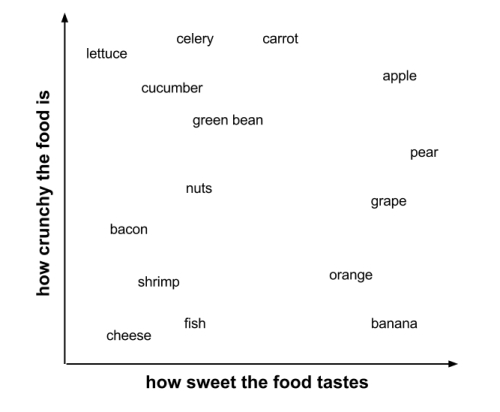
Did you notice the pattern? Similar types of food tend to be grouped closely together. As illustrated in the next figure, vegetables tend to be crunchy but not sweet, fruits tend to be sweet and either crunchy or not crunchy, while proteins tend to be neither crunchy nor sweet:

Suppose that after constructing this dataset, we decide to use it to settle the age-old question: is a tomato a fruit or a vegetable? We can use a nearest neighbor approach to determine which class is a better fit as shown in the following figure:

Locating the tomato's nearest neighbors requires a distance function, or a formula that measures the similarity between two instances.
There are many different ways to calculate distance. Traditionally, the kNN algorithm uses Euclidean distance, which is the distance one would measure if you could use a ruler to connect two points, illustrated in the previous figure by the dotted lines connecting the tomato to its neighbors.
Tip
Euclidean distance is measured "as the crow flies," implying the shortest direct route. Another common distance measure is
Manhattan distance, which is based on the paths a pedestrian would take by walking city blocks. If you are interested in learning more about other distance measures, you can read the documentation for R's distance function (a useful tool in its own right), using the ?dist command.
Euclidean distance is specified by the following formula, where p and q are the examples to be compared, each having n features. The term p1 refers to the value of the first feature of example p, while q1 refers to the value of the first feature of example q:

The distance formula involves comparing the values of each feature. For example, to calculate the distance between the tomato (sweetness = 6, crunchiness = 4), and the green bean (sweetness = 3, crunchiness = 7), we can use the formula as follows:

In a similar vein, we can calculate the distance between the tomato and several of its closest neighbors as follows:
|
ingredient |
sweetness |
crunchiness |
food type |
distance to the tomato |
|---|---|---|---|---|
|
grape |
8 |
5 |
fruit |
sqrt((6 - 8)^2 + (4 - 5)^2) = 2.2 |
|
green bean |
3 |
7 |
vegetable |
sqrt((6 - 3)^2 + (4 - 7)^2) = 4.2 |
|
nuts |
3 |
6 |
protein |
sqrt((6 - 3)^2 + (4 - 6)^2) = 3.6 |
|
orange |
7 |
3 |
fruit |
sqrt((6 - 7)^2 + (4 - 3)^2) = 1.4 |
To classify the tomato as a vegetable, protein, or fruit, we'll begin by assigning the tomato, the food type of its single nearest neighbor. This is called 1NN classification because k = 1. The orange is the nearest neighbor to the tomato, with a distance of 1.4. As orange is a fruit, the 1NN algorithm would classify tomato as a fruit.
If we use the kNN algorithm with k = 3 instead, it performs a vote among the three nearest neighbors: orange, grape, and nuts. Because the majority class among these neighbors is fruit (2 of the 3 votes), the tomato again is classified as a fruit.
Deciding how many neighbors to use for kNN determines how well the model will generalize to future data. The balance between overfitting and underfitting the training data is a problem known as the bias-variance tradeoff. Choosing a large k reduces the impact or variance caused by noisy data, but can bias the learner such that it runs the risk of ignoring small, but important patterns.
Suppose we took the extreme stance of setting a very large k, equal to the total number of observations in the training data. As every training instance is represented in the final vote, the most common training class always has a majority of the voters. The model would, thus, always predict the majority class, regardless of which neighbors are nearest.
On the opposite extreme, using a single nearest neighbor allows noisy data or outliers, to unduly influence the classification of examples. For example, suppose that some of the training examples were accidentally mislabeled. Any unlabeled example that happens to be nearest to the incorrectly labeled neighbor will be predicted to have the incorrect class, even if the other nine nearest neighbors would have voted differently.
Obviously, the best k value is somewhere between these two extremes.
The following figure illustrates more generally how the decision boundary (depicted by a dashed line) is affected by larger or smaller k values. Smaller values allow more complex decision boundaries that more carefully fit the training data. The problem is that we do not know whether the straight boundary or the curved boundary better represents the true underlying concept to be learned.

In practice, choosing k depends on the difficulty of the concept to be learned and the number of records in the training data. Typically, k is set somewhere between 3 and 10. One common practice is to set k equal to the square root of the number of training examples. In the food classifier we developed previously, we might set k = 4, because there were 15 example ingredients in the training data and the square root of 15 is 3.87.
However, such rules may not always result in the single best k. An alternative approach is to test several k values on a variety of test datasets and choose the one that delivers the best classification performance. On the other hand, unless the data is very noisy, larger and more representative training datasets can make the choice of k less important. This is because even subtle concepts will have a sufficiently large pool of examples to vote as nearest neighbors.
Features are typically transformed to a standard range prior to applying the kNN algorithm. The rationale for this step is that the distance formula is dependent on how features are measured. In particular, if certain features have much larger values than others, the distance measurements will be strongly dominated by the larger values. This wasn't a problem for us before with the food tasting data, as both sweetness and crunchiness were measured on a scale from 1 to 10.
Suppose that we added an additional feature indicating spiciness, which we measured using the Scoville scale. The Scoville scale is a standardized measure of spice heat, ranging from zero (not spicy) to over a million (for the hottest chili peppers). Because the difference between spicy foods and non-spicy foods can be over a million, while the difference between sweet and non-sweet is at most ten, we might find that our distance measures only differentiate foods by their spiciness; the impact of crunchiness and sweetness would be dwarfed by the contribution of spiciness.
What we need is a way of "shrinking" or rescaling the various features such that each one contributes relatively equally to the distance formula. For example, if sweetness and crunchiness are both measured on a scale from 1 to 10, we would also like spiciness to be measured on a scale from 1 to 10. There are several ways to accomplish such scaling.
The traditional method of rescaling features for kNN is min-max normalization. This process transforms a feature such that all of its values fall in a range between 0 and 1. The formula for normalizing a feature is as follows. Essentially, the formula subtracts the minimum of feature X from each value and divides by the range of X:

Normalized feature values can be interpreted as indicating how far, from 0 percent to 100 percent, the original value fell along the range between the original minimum and maximum.
Another common transformation is called z-score standardization. The following formula subtracts the mean value of feature X and divides by the standard deviation of X:
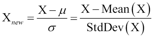
This formula, which is based on properties of the normal distribution covered in Chapter 2, Managing and Understanding Data, rescales each of a feature's values in terms of how many standard deviations they fall above or below the mean value. The resulting value is called a z-score. The z-scores fall in an unbounded range of negative and positive numbers. Unlike the normalized values, they have no predefined minimum and maximum.
The Euclidean distance formula is not defined for nominal data. Therefore, to calculate the distance between nominal features, we need to convert them into a numeric format. A typical solution utilizes dummy coding, where a value of 1 indicates one category, and 0 indicates the other. For instance, dummy coding for a gender variable could be constructed as:

Notice how dummy coding of the two-category (binary) gender variable results in a single new feature named male. There is no need to construct a separate feature for female; as the two sexes are mutually exclusive, knowing one or the other is enough.
This is true more generally as well. An n-category nominal feature can be dummy coded by creating binary indicator variables for (n - 1) levels of the feature. For example, dummy coding for a three-category temperature variable (for example, hot, medium, or cold) could be set up as (3 - 1) = 2 features, as shown:

Here, knowing that hot and medium are both 0 is enough to know that the temperature is cold. We, therefore, do not need a third feature for the cold attribute.
A convenient aspect of dummy coding is that the distance between dummy coded features is always one or zero, and thus, the values fall on the same scale as normalized numeric data. No additional transformation is necessary.
Tip
If your nominal feature is ordinal, (one could make such an argument for the temperature variable that we just saw) an alternative to dummy coding would be to number the categories and apply normalization. For instance, cold, warm, and hot could be numbered as 1, 2, and 3, which normalizes to 0, 0.5, and 1. A caveat to this approach is that it should only be used if you believe that the steps between categories are equivalent. For instance, you could argue that although, poor, middle class, and wealthy are ordered, the difference between poor and middle class is greater (or lesser) than the difference between middle class and wealthy. In this case, dummy coding is a safer approach.
Classification algorithms based on nearest neighbor methods are considered lazy learning algorithms because, technically speaking, no abstraction occurs. The abstraction and generalization processes are skipped altogether, which undermines the definition of learning presented in Chapter 1, Introducing Machine Learning.
Using the strict definition of learning, a lazy learner is not really learning anything. Instead, it merely stores the training data verbatim. This allows the training phase to occur very rapidly, with a potential downside being that the process of making predictions tends to be relatively slow. Due to the heavy reliance on the training instances, lazy learning is also known as instance-based learning or rote learning.
As instance-based learners do not build a model, the method is said to be in a class of non-parametric learning methods—no parameters are learned about the data. Without generating theories about the underlying data, non-parametric methods limit our ability to understand how the classifier is using the data. On the other hand, this allows the learner to find natural patterns rather than trying to fit the data into a preconceived form.
Although kNN classifiers may be considered lazy, they are still quite powerful. As you will soon see, the simple principles of kNN can be used to automate the process of screening for cancer.