The late science fiction author Arthur C. Clarke once wrote that "any sufficiently advanced technology is indistinguishable from magic." This chapter covers a pair of machine learning methods that may, likewise, appear at first glance to be magic. As two of the most powerful machine learning algorithms, they are applied to tasks across many domains. However, their inner workings can be difficult to understand.
In engineering, these are referred to as black box processes because the mechanism that transforms the input into the output is obfuscated by a figurative box. The reasons for the opacity can vary; for instance, black box closed source software intentionally conceals proprietary algorithms, the black box of sausage-making involves a bit of purposeful (but tasty) ignorance, and the black box of political lawmaking is rooted in bureaucratic processes. In the case of machine learning, the black box is because the underlying models are based on complex mathematical systems and the results are difficult to interpret.
Although it may not be feasible to interpret black box models, it is dangerous to apply the methods blindly. Therefore, in this chapter, we'll peek behind the curtain and investigate the statistical sausage-making involved in fitting such models. You'll discover that:
- Neural networks use concepts borrowed from an understanding of human brains in order to model arbitrary functions
- Support Vector Machines use multidimensional surfaces to define the relationship between features and outcomes
- In spite of their complexity, these models can be easily applied to real-world problems such as modeling the strength of concrete or reading printed text
With any luck, you'll realize that you don't need a black belt in statistics to tackle black box machine learning methods—there's no need to be intimidated!
An Artificial Neural Network (ANN) models the relationship between a set of input signals and an output signal using a model derived from our understanding of how a biological brain responds to stimuli from sensory inputs. Just as a brain uses a network of interconnected cells called neurons to create a massive parallel processor, the ANN uses a network of artificial neurons or nodes to solve learning problems.
The human brain is made up of about 85 billion neurons, resulting in a network capable of storing a tremendous amount of knowledge. As you might expect, this dwarfs the brains of other living creatures. For instance, a cat has roughly a billion neurons, a mouse has about 75 million neurons, and a cockroach has only about a million neurons. In contrast, many ANNs contain far fewer neurons, typically only several hundred, so we're in no danger of creating an artificial brain anytime in the near future—even a fruit fly brain with 100,000 neurons far exceeds the current ANN state-of-the-art.
Tip
Though it may be infeasible to completely model a cockroach's brain, a neural network might provide an adequate heuristic model of its behavior, such as in an algorithm that can mimic how a roach flees when discovered. If the behavior of a roboroach is convincing, does it matter how its brain works? This question is the basis of the controversial Turing test, which grades a machine as intelligent if a human being cannot distinguish its behavior from a living creature's.
Rudimentary ANNs have been used for over 50 years to simulate the brain's approach to problem solving. At first, this involved learning simple functions, like the logical AND function or the logical OR. These early exercises were used primarily to construct models of how biological brains might function. However, as computers have become increasingly powerful in recent years, the complexity of ANNs has likewise increased such that they are now frequently applied to more practical problems such as:
- Speech and handwriting recognition programs like those used by voicemail transcription services and postal mail sorting machines
- The automation of smart devices like an office building's environmental controls or self-driving cars and self-piloting drones
- Sophisticated models of weather and climate patterns, tensile strength, fluid dynamics, and many other scientific, social, or economic phenomena
Broadly speaking, ANNs are versatile learners that can be applied to nearly any learning task: classification, numeric prediction, and even unsupervised pattern recognition.
Tip
Whether deserving or not, ANN learners are often reported in the media with great fanfare. For instance, an "artificial brain" developed by Google was recently touted for its ability to identify cat videos on YouTube. Such hype may have less to do with anything unique to ANNs and more to do with the fact that ANNs are captivating because of their similarities to living minds.
ANNs are best applied to problems where the input data and output data are well-understood or at least fairly simple, yet the process that relates the input to output is extremely complex. As a black box method, they work well for these types of black box problems.
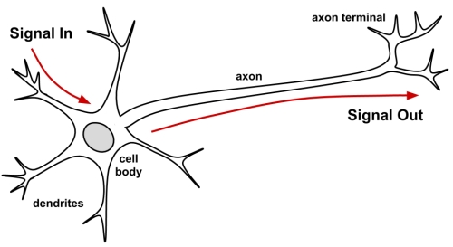
Because ANNs were intentionally designed as conceptual models of human brain activity, it is helpful to first understand how biological neurons function. As illustrated in the following figure, incoming signals are received by the cell's dendrites through a biochemical process that allows the impulse to be weighted according to its relative importance or frequency. As the cell body begins to accumulate the incoming signals, a threshold is reached at which the cell fires and the output signal is then transmitted via an electrochemical process down the axon. At the axon's terminals, the electric signal is again processed as a chemical signal to be passed to the neighboring neurons across a tiny gap known as a synapse.
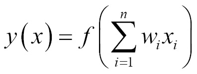
The model of a single artificial neuron can be understood in terms very similar to the biological model. As depicted in the following figure, a directed network diagram defines a relationship between the input signals received by the dendrites (x variables) and the output signal (y variable). Just as with the biological neuron, each dendrite's signal is weighted (w values) according to its importance—ignore for now how these weights are determined. The input signals are summed by the cell body and the signal is passed on according to an activation function denoted by f.

A typical artificial neuron with n input dendrites can be represented by the formula that follows. The w weights allow each of the n inputs, (x), to contribute a greater or lesser amount to the sum of input signals. The net total is used by the activation function f(x), and the resulting signal, y(x), is the output axon.
Neural networks use neurons defined in this way as building blocks to construct complex models of data. Although there are numerous variants of neural networks, each can be defined in terms of the following characteristics:
- An activation function, which transforms a neuron's net input signal into a single output signal to be broadcasted further in the network
- A network topology (or architecture), which describes the number of neurons in the model as well as the number of layers and manner in which they are connected
- The training algorithm that specifies how connection weights are set in order to inhibit or excite neurons in proportion to the input signal
Let's take a look at some of the variations within each of these categories to see how they can be used to construct typical neural network models.
The activation function is the mechanism by which the artificial neuron processes information and passes it throughout the network. Just as the artificial neuron is modeled after the biological version, so too is the activation function modeled after nature's design.
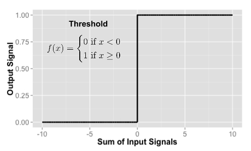
In the biological case, the activation function could be imagined as a process that involves summing the total input signal and determining whether it meets the firing threshold. If so, the neuron passes on the signal; otherwise, it does nothing. In ANN terms, this is known as a threshold activation function, as it results in an output signal only once a specified input threshold has been attained.
The following figure depicts a typical threshold function; in this case, the neuron fires when the sum of input signals is at least zero. Because of its shape, it is sometimes called a unit step activation function.
Although the threshold activation function is interesting due to its parallels with biology, it is rarely used in artificial neural networks. Freed from the limitations of biochemistry, ANN activation functions can be chosen based on their ability to demonstrate desirable mathematical characteristics and model relationships among data.
Perhaps the most commonly used alternative is the sigmoid activation function (specifically the logistic sigmoid) shown in the following figure, where e is the base of natural logarithms (approximately 2.72). Although it shares a similar step or S shape with the threshold activation function, the output signal is no longer binary; output values can fall anywhere in the range from 0 to 1. Additionally, the sigmoid is differentiable, which means that it is possible to calculate the derivative across the entire range of inputs. As you will learn later, this feature is crucial for creating efficient ANN optimization algorithms.

Although the sigmoid is perhaps the most commonly used activation function and is often used by default, some neural network algorithms allow a choice of alternatives. A selection of such activation functions is as shown:

The primary detail that differentiates among these activation functions is the output signal range. Typically, this is one of (0, 1), (-1, +1), or (-inf, +inf). The choice of activation function biases the neural network such that it may fit certain types of data more appropriately, allowing the construction of specialized neural networks. For instance, a linear activation function results in a neural network very similar to a linear regression model, while a Gaussian activation function results in a model called a Radial Basis Function (RBF) network.
It's important to recognize that for many of the activation functions, the range of input values that affect the output signal is relatively narrow. For example, in the case of the sigmoid, the output signal is always 0 or always 1 for an input signal below -5 or above +5, respectively. The compression of the signal in this way results in a saturated signal at the high and low ends of very dynamic inputs, just as turning a guitar amplifier up too high results in a distorted sound due to clipping the peaks of sound waves. Because this essentially squeezes the input values into a smaller range of outputs, such activation functions (like the sigmoid) are sometimes called squashing functions.
The solution to the squashing problem is to transform all neural network inputs such that the feature values fall within a small range around 0. Typically, this is done by standardizing or normalizing the features. By limiting the input values, the activation function will have action across the entire range, preventing large-valued features such as household income from dominating small-valued features such as the number of children in the household. A side benefit is that the model may also be faster to train, since the algorithm can iterate more quickly through the actionable range of input values.
Tip
Although theoretically a neural network can adapt to a very dynamic feature by adjusting its weight over many iterations, in extreme cases many algorithms will stop iterating long before this occurs. If your model is making predictions that do not make sense, double-check that you've correctly standardized the input data.
The capacity of a neural network to learn is rooted in its topology, or the patterns and structures of interconnected neurons. Although there are countless forms of network architecture, they can be differentiated by three key characteristics:
- The number of layers
- Whether information in the network is allowed to travel backward
- The number of nodes within each layer of the network
The topology determines the complexity of tasks that can be learned by the network. Generally, larger and more complex networks are capable of identifying more subtle patterns and complex decision boundaries. However, the power of a network is not only a function of the network size, but also the way units are arranged.
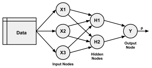
To define topology, we need a terminology that distinguishes artificial neurons based on their position in the network. The figure that follows illustrates the topology of a very simple network. A set of neurons called Input Nodes receive unprocessed signals directly from the input data. Each input node is responsible for processing a single feature in the dataset; the feature's value will be transformed by the node's activation function. The signals resulting from the input nodes are received by the Output Node, which uses its own activation function to generate a final prediction (denoted here as p).
The input and output nodes are arranged in groups known as layers. Because the input nodes process the incoming data exactly as received, the network has only one set of connection weights (labeled here as w1, w2, and w3). It is therefore termed a single-layer network. Single-layer networks can be used for basic pattern classification, particularly for patterns that are linearly separable, but more sophisticated networks are required for most learning tasks.

As you might expect, an obvious way to create more complex networks is by adding additional layers. As depicted here, a multilayer network adds one or more hidden layers that process the signals from the input nodes prior to reaching the output node. Most multilayer networks are fully connected, which means that every node in one layer is connected to every node in the next layer, but this is not required.
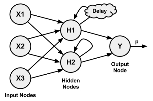
You may have noticed that in the prior examples arrowheads were used to indicate signals traveling in only one direction. Networks in which the input signal is fed continuously in one direction from connection-to-connection until reaching the output layer are called feedforward networks.
In spite of the restriction on information flow, feedforward networks offer a surprising amount of flexibility. For instance, the number of levels and nodes at each level can be varied, multiple outcomes can be modeled simultaneously, or multiple hidden layers can be applied (a practice that is sometimes referred to as deep learning).

In contrast, a recurrent network (or feedback network) allows signals to travel in both directions using loops. This property, which more closely mirrors how a biological neural network works, allows extremely complex patterns to be learned. The addition of a short term memory (labeled Delay in the following figure) increases the power of recurrent networks immensely. Notably, this includes the capability to understand sequences of events over a period of time. This could be used for stock market prediction, speech comprehension, or weather forecasting. A simple recurrent network is depicted as shown:
In spite of their potential, recurrent networks are still largely theoretical and are rarely used in practice. On the other hand, feedforward networks have been extensively applied to real-world problems. In fact, the multilayer feedforward network (sometimes called the Multilayer Perceptron (MLP) is the de facto standard ANN topology. If someone mentions that they are fitting a neural network without additional clarification, they are most likely referring to a multilayer feedforward network.
In addition to variations in the number of layers and the direction of information travel, neural networks can also vary in complexity by the number of nodes in each layer. The number of input nodes is predetermined by the number of features in the input data. Similarly, the number of output nodes is predetermined by the number of outcomes to be modeled or the number of class levels in the outcome. However, the number of hidden nodes is left to the user to decide prior to training the model.
Unfortunately, there is no reliable rule to determine the number of neurons in the hidden layer. The appropriate number depends on the number of input nodes, the amount of training data, the amount of noisy data, and the complexity of the learning task among many other factors.
In general, more complex network topologies with a greater number of network connections allow the learning of more complex problems. A greater number of neurons will result in a model that more closely mirrors the training data, but this runs a risk of overfitting; it may generalize poorly to future data. Large neural networks can also be computationally expensive and slow to train.
A best practice is to use the fewest nodes that result in adequate performance on a validation dataset. In most cases, even with only a small number of hidden nodes—often as few as a handful—the neural network can offer a tremendous amount of learning ability.
The network topology is a blank slate that by itself has not learned anything. Like a newborn child, it must be trained with experience. As the neural network processes the input data, connections between the neurons are strengthened or weakened similar to how a baby's brain develops as he or she experiences the environment. The network's connection weights reflect the patterns observed over time.
Training a neural network by adjusting connection weights is very computationally intensive. Consequently, though they had been studied for decades prior, ANNs were rarely applied to real-world learning tasks until the mid-to-late 1980s, when an efficient method of training an ANN was discovered. The algorithm, which used a strategy of back-propagating errors, is now known simply as backpropagation.
Although still notoriously slow relative to many other machine learning algorithms, the backpropagation method led to a resurgence of interest in ANNs. As a result, multilayer feedforward networks that use the backpropagation algorithm are now common in the field of data mining. Such models offer the following strengths and weaknesses:
|
Strengths |
Weaknesses |
|---|---|
In its most general form, the backpropagation algorithm iterates through many cycles of two processes. Each iteration of the algorithm is known as an epoch. Because the network contains no a priori (existing) knowledge, typically the weights are set randomly prior to beginning. Then, the algorithm cycles through the processes until a stopping criterion is reached. The cycles include:
- A forward phase in which the neurons are activated in sequence from the input layer to the output layer, applying each neuron's weights and activation function along the way. Upon reaching the final layer, an output signal is produced.
- A backward phase in which the network's output signal resulting from the forward phase is compared to the true target value in the training data. The difference between the network's output signal and the true value results in an error that is propagated backwards in the network to modify the connection weights between neurons and reduce future errors.
Over time, the network uses the information sent backward to reduce the total error of the network. Yet one question remains: because the relationship between each neuron's inputs and outputs is complex, how does the algorithm determine how much (or whether) a weight should be changed?
The answer to this question involves a technique called gradient descent. Conceptually, it works similarly to how an explorer trapped in the jungle might find a path to water. By examining the terrain and continually walking in the direction with the greatest downward slope, he or she is likely to eventually reach the lowest valley, which is likely to be a riverbed.
In a similar process, the backpropagation algorithm uses the derivative of each neuron's activation function to identify the gradient in the direction of each of the incoming weights—hence the importance of having a differentiable activation function. The gradient suggests how steeply the error will be reduced or increased for a change in the weight. The algorithm will attempt to change the weights that result in the greatest reduction in error by an amount known as the learning rate. The greater the learning rate, the faster the algorithm will attempt to descend down the gradients, which could reduce training time at the risk of overshooting the valley.
Although this process seems complex, it is easy to apply in practice. Let's apply our understanding of multilayer feedforward networks to a real-world problem.