In the field of engineering, it is crucial to have accurate estimates of the performance of building materials. These estimates are required in order to develop safety guidelines governing the materials used in the construction of buildings, bridges, and roadways.
Estimating the strength of concrete is a challenge of particular interest. Although it is used in nearly every construction project, concrete performance varies greatly due to the use of a wide variety of ingredients that interact in complex ways. As a result, it is difficult to accurately predict the strength of the final product. A model that could reliably predict concrete strength given a listing of the composition of the input materials could result in safer construction practices.
For this analysis, we will utilize data on the compressive strength of concrete donated to the UCI Machine Learning Data Repository (http://archive.ics.uci.edu/ml) by I-Cheng Yeh. As he found success using neural networks to model these data, we will attempt to replicate Yeh's work using a simple neural network model in R.
According to the website, the concrete dataset contains 1,030 examples of concrete, with eight features describing the components used in the mixture. These features are thought to be related to the final compressive strength, and they include the amount (in kilograms per cubic meter) of cement, slag, ash, water, superplasticizer, coarse aggregate, and fine aggregate used in the product, in addition to the aging time (measured in days).
As usual, we'll begin our analysis by loading the data into an R object using the read.csv() function and confirming that it matches the expected structure:
> concrete <- read.csv("concrete.csv")
> str(concrete)
'data.frame':	1030 obs. of  9 variables:
 $ cement      : num  141 169 250 266 155 ...
 $ slag        : num  212 42.2 0 114 183.4 ...
 $ ash         : num  0 124.3 95.7 0 0 ...
 $ water       : num  204 158 187 228 193 ...
 $ superplastic: num  0 10.8 5.5 0 9.1 0 0 6.4 0 9 ...
 $ coarseagg   : num  972 1081 957 932 1047 ...
 $ fineagg     : num  748 796 861 670 697 ...
 $ age         : int  28 14 28 28 28 90 7 56 28 28 ...
 $ strength    : num  29.9 23.5 29.2 45.9 18.3 ...
The nine variables in the data frame correspond to the eight features and one outcome we expected, although a problem has become apparent. Neural networks work best when the input data are scaled to a narrow range around zero, and here we see values ranging anywhere from zero up to over a thousand.
Typically, the solution to this problem is to rescale the data with a normalizing or standardization function. If the data follow a bell-shaped curve (a normal distribution as described in Chapter 2, Managing and Understanding Data), then it may make sense to use standardization via R's built-in scale() function. On the other hand, if the data follow a uniform distribution or are severely non-normal, then normalization to a 0-1 range may be more appropriate. In this case, we'll use the latter.
In Chapter 3, Lazy Learning – Classification Using Nearest Neighbors, we defined our own normalize() function as:
> normalize <- function(x) {
    return((x - min(x)) / (max(x) - min(x)))
  }
After executing this code, our normalize() function can be applied to every column in the concrete data frame using the lapply() function as follows:
> concrete_norm <- as.data.frame(lapply(concrete, normalize))
To confirm that the normalization worked, we can see that the minimum and maximum strength are now 0 and 1, respectively:
> summary(concrete_norm$strength)
     Min.   1st Qu.    Median      Mean   3rd Qu.      Max.
0.0000000 0.2663511 0.4000872 0.4171915 0.5457207 1.0000000
In comparison, the original minimum and maximum values were 2.33 and 82.6:
> summary(concrete$strength)
    Min.  1st Qu.   Median     Mean  3rd Qu.     Max.
 2.33000 23.71000 34.44500 35.81796 46.13500 82.60000
Tip
Any transformation applied to the data prior to training the model will have to be applied in reverse later on in order to convert back to the original units of measurement. To facilitate the rescaling, it is wise to save the original data, or at least the summary statistics of the original data.
Following the precedent of I-Cheng Yeh in the original publication, we will partition the data into a training set with 75 percent of the examples and a testing set with 25 percent. The CSV file we used was already sorted in random order, so we simply need to divide it into two portions:
> concrete_train <- concrete_norm[1:773, ]
> concrete_test <- concrete_norm[774:1030, ]
We'll use the training dataset to build the neural network and the testing dataset to evaluate how well the model generalizes to future results. As it is easy to overfit a neural network, this step is very important.
To model the relationship between the ingredients used in concrete and the strength of the finished product, we will use a multilayer feedforward neural network. The neuralnet package by Stefan Fritsch and Frauke Guenther provides a standard and easy-to-use implementation of such networks. It also offers a function to plot the network topology. For these reasons, the neuralnet implementation is a strong choice for learning more about neural networks, though that's not to say that it cannot be used to accomplish real work as well—it's quite a powerful tool, as you will soon see.
Tip
There are several other commonly used packages to train ANN models in R, each with unique strengths and weaknesses. Because it ships as part of the standard R installation, the nnet package is perhaps the most frequently cited ANN implementation. It uses a slightly more sophisticated algorithm than standard backpropagation. Another strong option is the RSNNS package, which offers a complete suite of neural network functionality, with the downside being that it is more difficult to learn.
As neuralnet is not included in base R, you will need to install it by typing install.packages("neuralnet") and load it with the library(neuralnet) command. The included neuralnet() function can be used for training neural networks for numeric prediction using the following syntax:
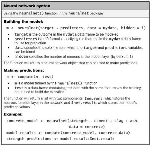
We'll begin by training the simplest multilayer feedforward network with only a single hidden node:
> concrete_model <- neuralnet(strength ~ cement + slag +
                              ash + water + superplastic +
                              coarseagg + fineagg + age,
                              data = concrete_train)
We can then visualize the network topology using the plot() function on the concrete_model object:
> plot(concrete_model)

In this simple model, there is one input node for each of the eight features, followed by a single hidden node and a single output node that predicts the concrete strength. The weights for each of the connections are also depicted, as are the bias terms (indicated by the nodes with a 1). The plot also reports the number of training steps and a measure called, the Sum of Squared Errors (SSE). These metrics will be useful when we are evaluating the model performance.
The network topology diagram gives us a peek into the black box of the ANN, but it doesn't provide much information about how well the model fits our data. To estimate our model's performance, we can use the compute() function to generate predictions on the testing dataset:
> model_results <- compute(concrete_model, concrete_test[1:8])
Note that the compute() function works a bit differently from the predict() functions we've used so far. It returns a list with two components: $neurons, which stores the neurons for each layer in the network, and $net.results, which stores the predicted values. We'll want the latter:
> predicted_strength <- model_results$net.result
Because this is a numeric prediction problem rather than a classification problem, we cannot use a confusion matrix to examine model accuracy. Instead, we must measure the correlation between our predicted concrete strength and the true value. This provides an insight into the strength of the linear association between the two variables.
Recall that the cor() function is used to obtain a correlation between two numeric vectors:
> cor(predicted_strength, concrete_test$strength)
             [,1]
[1,] 0.7170368646
Correlations close to 1 indicate strong linear relationships between two variables. Therefore, the correlation here of about 0.72 indicates a fairly strong relationship. This implies that our model is doing a fairly good job, even with only a single hidden node.
Tip
A neural network with a single hidden node can be thought of as a distant cousin of the linear regression models we studied in Chapter 6, Forecasting Numeric Data – Regression Methods. The weight between each input node and the hidden node is similar to the regression coefficients, and the weight for the bias term is similar to the intercept. In fact, if you construct a linear model in the same vein as the previous ANN, the correlation is 0.74.
Given that we only used one hidden node, it is likely that we can improve the performance of our model. Let's try to do a bit better.
As networks with more complex topologies are capable of learning more difficult concepts, let's see what happens when we increase the number of hidden nodes to five. We use the neuralnet() function as before, but add the parameter hidden = 5:
> concrete_model2 <- neuralnet(strength ~ cement + slag +
                               ash + water + superplastic +
                               coarseagg + fineagg + age,
                               data = concrete_train, hidden = 5)
Plotting the network again, we see a drastic increase in the number of connections. How did this impact performance?
> plot(concrete_model2)
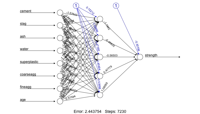
Notice that the reported error (measured again by SSE) has been reduced from 6.92 in the previous model to 2.44 here. Additionally, the number of training steps rose from 3222 to 7230, which is no surprise given how much more complex the model has become.
Applying the same steps to compare the predicted values to the true values, we now obtain a correlation around 0.80, which is a considerable improvement over the previous result:
> model_results2 <- compute(concrete_model2, concrete_test[1:8])
> predicted_strength2 <- model_results2$net.result
> cor(predicted_strength2, concrete_test$strength)
            [,1]
[1,] 0.801444583
Interestingly, in the original publication, I-Cheng Yeh reported a mean correlation of 0.885 using a very similar neural network. For some reason, we fell a bit short. In our defense, he is a civil engineering professor; therefore, he may have applied some subject matter expertise to the data preparation. If you'd like more practice with neural networks, you might try applying the principles learned earlier in this chapter to beat his result, perhaps by using different numbers of hidden nodes, applying different activation functions, and so on. The ?neuralnet help page provides more information on the various parameters that can be adjusted.