Our market basket analysis will utilize purchase data from one month of operation at a real-world grocery store. The data contain 9,835 transactions, or about 327 transactions per day (roughly 30 transactions per hour in a 12 hour business day), suggesting that the retailer is not particularly large, nor is it particularly small.

In a typical grocery store, there is a huge variety of items. There might be five brands of milk, a dozen different types of laundry detergent, and three brands of coffee. Given the moderate size of the retailer, we will assume that they are not terribly concerned with finding rules that apply only to a specific brand of milk or detergent. With this in mind, all brand names can be removed from the purchases. This reduces the number of groceries to a more manageable 169 types, using broad categories such as chicken, frozen meals, margarine, and soda.

Do you have any guesses about which types of items might be purchased together? Will wine and cheese be a common pairing? Bread and butter? Tea and honey? Let's dig into this data and see if we can confirm our guesses.

Unlike the datasets we've used previously, transactional data is stored in a slightly different format. Most of our prior analyses utilized data in the form of a matrix where rows indicated example instances and columns indicated features. Given the structure of the matrix format, all examples are required to have exactly the same set of features.

In comparison, transactional data is more free-form. As usual, each row in the data specifies a single example—in this case, a transaction. However, rather than having a set number of features, each record comprises a comma-separated list of any number of items, from one to many. In essence, the features may differ from example to example.

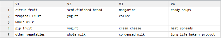
The first five rows of the raw grocery.csv data are as follows:

citrus fruit,semi-finished bread,margarine,ready soups
tropical fruit,yogurt,coffee
whole milk
pip fruit,yogurt,cream cheese,meat spreads
other vegetables,whole milk,condensed milk,long life bakery product

These lines indicate five separate grocery store transactions. The first transaction included four items: citrus fruit, semi-finished bread, margarine, and ready soups. In comparison, the third transaction included only one item, whole milk.

Suppose we tried to load the data using the read.csv() function as we had done in prior analyses. R would happily comply and read the data into a matrix form as follows:

You will notice that R created four variables to store the items in the transactional data: V1, V2, V3, and V4. Although it was nice of R to do this, if we use the data like this, we will encounter problems later on. First, R chose to create four variables because the first line had exactly four comma-separated values. However, we know that grocery purchases can contain more than four items; these transactions unfortunately will be broken across multiple rows in the matrix. We could try to remedy this by putting the transaction with the largest number of items at the top of the file, but this ignores another, more problematic issue.

The problem is due to the fact that by structuring the data this way, R has constructed a set of features that record not just the items in the transactions, but also the order they appear. If we imagine our learning algorithm as an attempt to find a relationship among V1, V2, V3, and V4, then whole milk in V1 might be treated differently than whole milk appearing in V2. Instead, we need a dataset that does not treat a transaction as a set of positions to be filled (or not filled) with specific items, but rather as a market basket that either contains or does not contain each particular item.

> groceries <- read.transactions("groceries.csv", sep = ",")

> summary(groceries)
transactions as itemMatrix in sparse format with
 9835 rows (elements/itemsets/transactions) and
 169 columns (items) and a density of 0.02609146

most frequent items:
      whole milk other vegetables       rolls/buns 
            2513             1903             1809 
            soda           yogurt          (Other) 
            1715             1372            34055 

element (itemset/transaction) length distribution:
sizes
   1    2    3    4    5    6    7    8    9   10   11   12 
2159 1643 1299 1005  855  645  545  438  350  246  182  117 
  13   14   15   16   17   18   19   20   21   22   23   24 
  78   77   55   46   29   14   14    9   11    4    6    1 
  26   27   28   29   32 
   1    1    1    3    1 

   Min. 1st Qu.  Median    Mean 3rd Qu.    Max. 
  1.000   2.000   3.000   4.409   6.000  32.000

> inspect(groceries[1:5])
  items                     
1 {citrus fruit,            
   margarine,               
   ready soups,             
   semi-finished bread}     
2 {coffee,                  
   tropical fruit,          
   yogurt}                  
3 {whole milk}              
4 {cream cheese,            
   meat spreads,            
   pip fruit,               
   yogurt}                  
5 {condensed milk,          
   long life bakery product,
   other vegetables,        
   whole milk}

> itemFrequency(groceries[, 1:3])
abrasive cleaner artif. sweetener   baby cosmetics 
    0.0035587189     0.0032536858     0.0006100661

Visualizing item support – item frequency plots

To present these statistics visually, use the itemFrequencyPlot() function. This allows you to produce at a bar chart depicting the proportion of transactions containing certain items. Since transactional data contains a very large number of items, you will often need to limit those appearing in the plot in order to produce a legible chart.

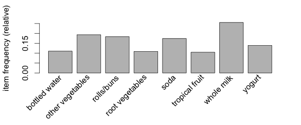
If you would like to require those items to appear in a minimum proportion of transactions, use itemFrequencyPlot() with the support parameter:

> itemFrequencyPlot(groceries, support = 0.1)

As shown in the following plot, this results in a histogram showing the eight items in the groceries data with at least 10 percent support:

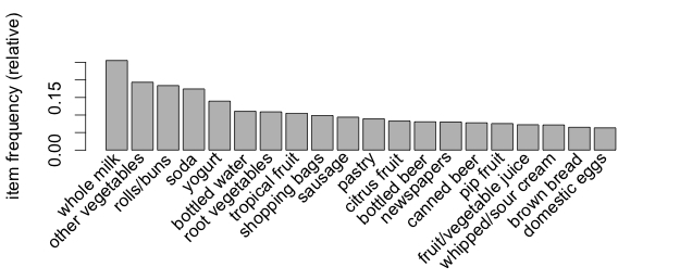
If you would rather limit the plot to a specific number of items, the topN parameter can be used with itemFrequencyPlot():

> itemFrequencyPlot(groceries, topN = 20)

The histogram is then sorted by decreasing support, as shown in the following diagram for the top 20 items in the groceries data:

Visualizing transaction data – plotting the sparse matrix

In addition to looking at items, it's also possible to visualize the entire sparse matrix. To do so, use the image() function. The sparse matrix for the first five transactions is as follows:

> image(groceries[1:5])

The resulting diagram depicts a matrix with five rows and 169 columns, indicating the five transactions and 169 possible items we requested. Cells in the matrix are filled with black for transactions (rows) where the item (column) was purchased.

Although the figure is small and may be slightly hard to read, you can see that the first, fourth, and fifth transactions contained four items each, since their rows have four cells filled in. You can also see that rows three, five, two, and four have an item in common (on the right side of the diagram).

This visualization can be a useful tool for exploring the data. For one, it may help with the identification of potential data issues. Columns that are filled all the way down could indicate items that are purchased in every transaction—a problem that could arise, perhaps, if a retailer's name or identification number was inadvertently included in the transaction dataset.

Additionally, patterns in the diagram may help reveal interesting segments of transactions or items, particularly if the data is sorted in interesting ways. For example, if the transactions are sorted by date, patterns in the black dots could reveal seasonal effects in the number or types of items people purchase. Perhaps around Christmas or Hanukkah, toys are more common; around Halloween, perhaps candy becomes popular. This type of visualization could be especially powerful if the items were also sorted into categories. In most cases, however, the plot will look fairly random, like static on a television screen.

Keep in mind that this visualization will not be as useful for extremely large transaction databases because the cells will be too small to discern. Still, by combining it with the sample() function, you can view the sparse matrix for a randomly sampled set of transactions. Here is what a random selection of 100 transactions looks like:

> image(sample(groceries, 100))

This creates a matrix diagram with 100 rows and the same 169 columns, as follows:

A few columns seem fairly heavily populated, indicating some very popular items at the store, but overall, the distribution of dots seems fairly random. Given nothing else of note, let's continue with our analysis.

With data preparation taken care of, we can now work at finding the associations among shopping cart items. We will use an implementation of the Apriori algorithm in the arules package we've been using for exploring and preparing the groceries data. You'll need to install and load this package if you have not done so already. The following table shows the syntax for creating sets of rules with the apriori() function:

Although running the apriori() function is straightforward, there can sometimes be a fair amount of trial and error when finding support and confidence parameters to produce a reasonable number of association rules. If you set these levels too high, then you might find no rules or rules that are too generic to be very useful. On the other hand, a threshold too low might result in an unwieldy number of rules, or worse, the operation might take a very long time or run out of memory during the learning phase.

In this case, if we attempt to use the default settings of support = 0.1 and confidence = 0.8, we end up with a set of zero rules:

> apriori(groceries)
set of 0 rules

Obviously, we need to widen the search a bit.

One way to approach the problem of setting support is to think about the minimum number of transactions you would need before you would consider a pattern interesting. For instance, you could argue that if an item is purchased twice a day (about 60 times) then it may be worth taking a look at. From there, it is possible to calculate the support level needed to find only rules matching at least that many transactions. Since 60 out of 9,835 equals 0.006, we'll try setting the support there first.

Setting the minimum confidence involves a tricky balance. On one hand, if confidence is too low, then we might be overwhelmed with a large number of unreliable rules—such as dozens of rules indicating items commonly purchased with batteries. How would we know where to target our advertising budget then? On the other hand, if we set confidence too high, then we will be limited to rules that are obvious or inevitable—like the fact that a smoke detector is always purchased in combination with batteries. In this case, moving the smoke detectors closer to the batteries is unlikely to generate additional revenue, since the two items were already almost always purchased together.

We'll start with a confidence threshold of 0.25, which means that in order to be included in the results, the rule has to be correct at least 25 percent of the time. This will eliminate the most unreliable rules while allowing some room for us to modify behavior with targeted promotions.

We are now ready to generate some rules. In addition to the minimum support and confidence, it is helpful to set minlen = 2 to eliminate rules that contain fewer than two items. This prevents uninteresting rules from being created simply because the item is purchased frequently, for instance, {} => whole milk. This rule meets the minimum support and confidence because whole milk is purchased in over 25 percent of transactions, but it isn't a very actionable rule.

The full command for finding a set of association rules using the Apriori algorithm is as follows:

> groceryrules <- apriori(groceries, parameter = list(support = 
                            0.006, confidence = 0.25, minlen = 2))

This saves our rules in a rules object, which we can peek into by typing its name:

> groceryrules
set of 463 rules

Our groceryrules object contains a set of 463 association rules. To determine whether any of them are useful, we'll have to dig deeper.

To obtain a high-level overview of the association rules, we can use summary() as follows. The rule length distribution tells us how many rules have each count of items. In our rule set, 150 rules have only two items, while 297 have three, and 16 have four. The summary statistics associated with this distribution are also given:

> summary(groceryrules)
set of 463 rules

rule length distribution (lhs + rhs):sizes
  2   3   4 
150 297  16 

   Min. 1st Qu.  Median    Mean 3rd Qu.    Max. 
  2.000   2.000   3.000   2.711   3.000   4.000 

Next, we see summary statistics for the rule quality measures: support, confidence, and lift. Support and confidence should not be very surprising, since we used these as selection criteria for the rules. However, we might be alarmed if most or all of the rules were very near the minimum thresholds—not the case here.

summary of quality measures:
    support           confidence          lift       
 Min.   :0.006101   Min.   :0.2500   Min.   :0.9932  
 1st Qu.:0.007117   1st Qu.:0.2971   1st Qu.:1.6229  
 Median :0.008744   Median :0.3554   Median :1.9332  
 Mean   :0.011539   Mean   :0.3786   Mean   :2.0351  
 3rd Qu.:0.012303   3rd Qu.:0.4495   3rd Qu.:2.3565  
 Max.   :0.074835   Max.   :0.6600   Max.   :3.9565  

The third column, lift, is a metric we have not considered yet. It is a measure of how much more likely one item is to be purchased relative to its typical purchase rate, given that you know another item has been purchased. This is defined by the following equation:

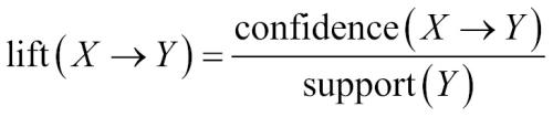
For example, suppose at a grocery store, most people purchase milk and bread. By chance alone, we would expect to find many transactions with both milk and bread. However, if lift(milk -> bread) is greater than 1, this implies that the two items are found together more often than one would expect by chance. A large lift value is therefore a strong indicator that a rule is important, and reflects a true connection between the items.

In the final section of the summary() output, we receive mining information, telling us about how the rules were chosen. Here, we see that the groceries data, which contained 9,835 transactions, was used to construct rules with a minimum support of 0.006 and minimum confidence of 0.25:

mining info:
      data ntransactions support confidence
 groceries          9835   0.006       0.25

We can take a look at specific rules using the inspect() function. For instance, the first three rules in the groceryrules object can be viewed as follows:

> inspect(groceryrules[1:3])

The columns indicated by lhs and rhs refer to the left-hand side (LHS) and right-hand side (RHS) of the rule. The LHS is the condition that needs to be met in order to trigger the rule, and the RHS is the expected result of meeting that condition.

The first rule can be read in plain language as "if a customer buys potted plants, they will also buy whole milk." With a support of about 0.007 and confidence of 0.400, we can determine that this rule covers about 0.7 percent of transactions, and is correct in 40 percent of purchases involving potted plants. The lift value tells us how much more likely a customer is to buy whole milk relative to the average customer, given that he or she bought a potted plant. Since we know that about 25.6 percent of customers bought whole milk (the support) while 40 percent of customers buying a potted plant bought whole milk (the confidence), we can compute the lift as 0.40 / 0.256 = 1.56, which matches the value shown. (Note that the column labeled support indicates the support for the rule, not the support for the lhs or rhs).

In spite of the fact that the confidence and lift are high, does {potted plants} => {whole milk} seem like a very useful rule? Probably not—there doesn't seem to be a logical reason why someone would be more likely to buy milk with a potted plant. Yet our data suggests otherwise. How can we make sense of this fact?

A common approach is to take the result of learning association rules and divide them into three categories:

Obviously, the goal of a market basket analysis is to find actionable associations, or rules that provide a clear and useful insight. Some rules are clear, others are useful; it is less common to find a combination of both of these factors.

Trivial rules include any rules that are so obvious that they are not worth mentioning—they are clear, but not useful. Suppose you were a marketing consultant being paid large sums of money to identify new opportunities for cross-promoting items. If you report the finding that {diapers} => {formula}, you probably won't be invited back for another consulting job.

Rules are inexplicable if the connection between the items is so unclear that figuring out how to use the information for action would require additional research. The rule may simply be a random pattern in the data, for instance, a rule stating that {pickles} => {chocolate ice cream} may be due to a single customer whose pregnant wife had regular cravings for strange combinations of foods.

The best rules are the hidden gems—those undiscovered insights into patterns that seem obvious once discovered. Given enough time, one could evaluate each of the 463 rules to find the gems. However, we (the one performing the market basket analysis) may not be the best judge of whether a rule is actionable, trivial, or inexplicable. In the next section, we'll improve the utility of our work by employing methods for sorting and sharing the learned rules so that the most interesting results might float to the top.

Subject matter experts may be able to identify useful rules very quickly, but it would be a poor use of their time to ask them to evaluate hundreds or thousands of rules. Therefore, it's useful to be able to sort the rules according to different criteria and get them out of R into a form that can be shared with marketing teams and examined in more depth. In this way, we can improve the performance of our rules by making the results more actionable.

Sorting the set of association rules

Depending upon the objectives of the market basket analysis, the most useful rules might be those with the highest support, confidence, or lift. The arules package includes a sort() function that can be used to reorder the list of rules so that those with the highest or lowest values of the quality measure come first.

To reorder the groceryrules, we can apply sort() while specifying a by parameter of "support", "confidence", or "lift". By combining the sort with vector operators, we can obtain a specific number of interesting rules. For instance, the best five rules according to the lift statistic can be examined using the following command:

> inspect(sort(groceryrules, by = "lift")[1:5])

This will look like the following screenshot:

These appear to be more interesting rules than the ones we looked at previously. The first rule, with a lift of 3.956477, implies that people who buy herbs are nearly four times more likely to buy root vegetables than the typical customer—perhaps for a stew of some sort? Rule two is also interesting. Whipped cream is over three times more likely to be found in a shopping cart with berries versus other carts, suggesting perhaps a dessert pairing?

Tip

By default, the sort order is decreasing, meaning the largest values come first. To reverse this order, add an additional parameter decreasing = FALSE.

Taking subsets of association rules

Suppose that given the preceding rule, the marketing team is excited about the possibilities of creating an advertisement to promote berries, which are now in season. Before finalizing the campaign, however, they ask you to investigate whether berries are often purchased with other items. To answer this question, we'll need to find all the rules that include berries in some form.

The subset() function provides a method for searching for subsets of transactions, items, or rules. To use it to find any rules with berries appearing in the rule, use the following command. This will store the rules in a new object titled berryrules:

> berryrules <- subset(groceryrules, items %in% "berries")

We can then inspect the rules as we had done with the larger set:

> inspect(berryrules)

The result is the folllowing set of rules:

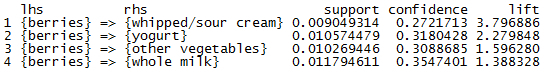
There are four rules involving berries, two of which seem to be interesting enough to call actionable. In addition to whipped cream, berries are also purchased frequently with yogurt—a pairing that could serve well for breakfast or lunch as well as dessert.

The subset() function is very powerful. The criteria for choosing the subset can be defined with several keywords and operators:

• The keyword items, explained previously, matches an item appearing anywhere in the rule. To limit the subset to where the match occurs only on the left or right-hand side, use lhs and rhs instead.
• The operator %in% means that at least one of the items must be found in the list you defined. If you wanted any rules matching either berries or yogurt, you could write items %in% c("berries", "yogurt").
• Additional operators are available for partial matching (%pin%) and complete matching (%ain%). Partial matching allows you to find both citrus fruit and tropical fruit using one search: items %pin% "fruit". Complete matching requires that all listed items are present. For instance, items %ain% c("berries", "yogurt") finds only rules with both berries and yogurt.
• Subsets can also be limited by support, confidence, or lift. For instance, confidence > 0.50 would limit you to rules with confidence greater than 50 percent.
• Matching criteria can be combined with standard R logical operators such as and (&), or (|), and not (!).

Using these options, you can limit the selection of rules to be as specific or general as you would like.

> write(groceryrules, file = "groceryrules.csv",
        sep = ",", quote = TRUE, row.names = FALSE)

> groceryrules_df <- as(groceryrules, "data.frame")

> str(groceryrules_df)
'data.frame':	463 obs. of 4 variables:
 $ rules     : Factor w/ 463 levels "{baking powder} => {other vegetables}",..: 340 302 207 206 208 341 402 21 139 140 ...
 $ support   : num  0.00691 0.0061 0.00702 0.00773 0.00773 ...
 $ confidence: num  0.4 0.405 0.431 0.475 0.475 ...
 $ lift      : num  1.57 1.59 3.96 2.45 1.86 ...