A Support Vector Machine (SVM) can be imagined as a surface that defines a boundary between various points of data which represent examples plotted in multidimensional space according to their feature values. The goal of an SVM is to create a flat boundary, called a hyperplane, which leads to fairly homogeneous partitions of data on either side. In this way, SVM learning combines aspects of both the instance-based nearest neighbor learning presented in Chapter 3, Lazy Learning – Classification Using Nearest Neighbors, and the linear regression modeling described in Chapter 6, Forecasting Numeric Data – Regression Methods. The combination is extremely powerful, allowing SVMs to model highly complex relationships.
Although the basic mathematics that drive SVMs have been around for decades, they have recently exploded in popularity. This is of course rooted in their state-of-the-art performance, but perhaps also due to the fact that award winning SVM algorithms have been implemented in several popular and well-supported libraries across many programming languages, including R. This has led SVMs to be adopted by a much wider audience who previously might have passed it by due to the somewhat complex math involved with SVM implementation. The good news is that although the math may be difficult, the basic concepts are understandable.
SVMs can be adapted for use with nearly any type of learning task, including both classification and numeric prediction. Many of the algorithm's key successes have come in pattern recognition. Notable applications include:
- Classification of microarray gene expression data in the field of bioinformatics to identify cancer or other genetic diseases
- Text categorization, such as identification of the language used in a document or organizing documents by subject matter
- The detection of rare yet important events like combustion engine failure, security breaches, or earthquakes
SVMs are most easily understood when used for binary classification, which is how the method has been traditionally applied. Therefore, in the remaining sections we will focus only on SVM classifiers. Don't worry, however, as the same principles you learn here will apply when adapting SVMs to other learning tasks such as numeric prediction.
As noted previously, SVMs use a linear boundary called a hyperplane to partition data into groups of similar elements, typically as indicated by the class values. For example, the following figure depicts a hyperplane that separates groups of circles and squares in two and three dimensions. Because the circles and squares can be divided by the straight line or flat surface, they are said to be linearly separable. At first, we'll consider only the simple case where this is true, but SVMs can also be extended to problems were the data are not linearly separable.

Tip
For convenience, the hyperplane is traditionally depicted as a line in 2D space, but this is simply because it is difficult to illustrate space in greater than two dimensions. In reality, the hyperplane is a flat surface in a high-dimensional space—a concept that can be difficult to get your mind around.
The task of the SVM algorithm is to identify a line that separates the two classes. As shown in the following figure, there is more than one choice of dividing line between the groups of circles and squares. Three such possibilities are labeled a, b, and c. How does the algorithm choose?
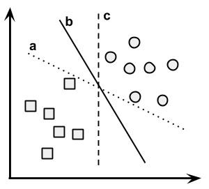
The answer to that question involves a search for the Maximum Margin Hyperplane (MMH) that creates the greatest separation between the two classes. Although any of the three lines separating the circles and squares would correctly classify all the data points, it is likely that the line that leads to the greatest separation will generalize the best to future data. This is because slight variations in the positions of the points near the boundary might cause one of them to fall over the line by chance.
The support vectors (indicated by arrows in the figure that follows) are the points from each class that are the closest to the MMH; each class must have at least one support vector, but it is possible to have more than one. Using the support vectors alone, it is possible to define the MMH. This is a key feature of SVMs; the support vectors provide a very compact way to store a classification model, even if the number of features is extremely large.

The algorithm to identify the support vectors relies on vector geometry and involves some fairly tricky math which is outside the scope of this book. However, the basic principles of the process are fairly straightforward.
Note
More information on the mathematics of SVMs can be found in the classic paper: Support-vector network, Machine Learning, Vol. 20, pp. 273-297, by C. Cortes and V. Vapnik (1995). A beginner level discussion can be found in Support vector machines: hype or hallelujah, SIGKDD Explorations, Vol. 2, No. 2, pp. 1-13, by K.P. Bennett and C. Campbell (2003). A more in-depth look can be found in: Support Vector Machines by I. Steinwart and A. Christmann (Springer Publishing Company, 2008).
It is easiest to understand how to find the maximum margin under the assumption that the classes are linearly separable. In this case, the MMH is as far away as possible from the outer boundaries of the two groups of data points. These outer boundaries are known as the convex hull. The MMH is then the perpendicular bisector of the shortest line between the two convex hulls. Sophisticated computer algorithms that use a technique known as quadratic optimization are capable of finding the maximum margin in this way.

An alternative (but equivalent) approach involves a search through the space of every possible hyperplane in order to find a set of two parallel planes which divide the points into homogeneous groups yet themselves are as far apart as possible. Stated differently, this process is a bit like trying to find the largest mattress that can fit up the stairwell to your bedroom.
To understand this search process, we'll need to define exactly what we mean by a hyperplane. In n-dimensional space, the following equation is used:
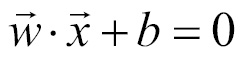
If you aren't familiar with this notation, the arrows above the letters indicate that they are vectors rather than single numbers. In particular, w is a vector of n weights, that is, {w1, w2, …, wn}, and b is a single number known as the bias.
Using this formula, the goal of the process is to find a set of weights that specify two hyperplanes, as follows:

We will also require that these hyperplanes are specified such that all the points of one class fall above the first hyperplane and all the points of the other class fall beneath the second hyperplane. This is possible so long as the data are linearly separable.
Vector geometry defines the distance between these two planes as:
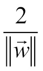
Here, ||w|| indicates the Euclidean norm (the distance from the origin to vector w). Therefore, in order to maximize distance, we need to minimize ||w||. In order to facilitate finding the solution, the task is typically reexpressed as a set of constraints:

Although this looks messy, it's really not too complicated if you think about it in pieces. Basically, the idea is to minimize the previous formula subject to (s.t.) the condition each of the y i data points is correctly classified. Note that y indicates the class value (transformed to either +1 or -1) and the upside down "A" is shorthand for "for all."
As with the other method for finding the maximum margin, finding a solution to this problem is a job for quadratic optimization software. Although it can be processor-intensive, specialized algorithms are capable of solving these problems quickly even on fairly large datasets.
As we've worked through the theory behind SVMs, you may be wondering about the elephant in the room: what happens in the case that the data are not linearly separable? The solution to this problem is the use of a slack variable, which creates a soft margin that allows some points to fall on the incorrect side of the margin. The figure that follows illustrates two points falling on the wrong side of the line with the corresponding slack terms (denoted with the Greek letter Xi):

A cost value (denoted as C) is applied to all points that violate the constraints, and rather than finding the maximum margin, the algorithm attempts to minimize the total cost. We can therefore revise the optimization problem to:
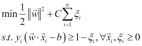
If you're confused by now, don't worry, you're not alone. Luckily, SVM packages will happily optimize this for you without you having to understand the technical details. The important piece to understand is the addition of the cost parameter, C. Modifying this value will adjust the penalty for examples that fall on the wrong side of the hyperplane. The greater the cost parameter, the harder the optimization will try to achieve 100 percent separation. On the other hand, a lower cost parameter will place the emphasis on a wider overall margin. It is important to strike a balance between these two in order to create a model that generalizes well to future data.
In many real-world applications, the relationships between variables are non-linear. As we just discovered, a SVM can still be trained on such data through the addition of a slack variable, which allows some examples to be misclassified. However, this is not the only way to approach the problem of non-linearity. A key feature of SVMs is their ability to map the problem into a higher dimension space using a process known as the kernel trick. In doing so, a non-linear relationship may suddenly appear to be quite linear.
Though this seems like nonsense, it is actually quite easy to illustrate by example. In the following figure, the scatterplot on the left depicts a non-linear relationship between a weather class (sunny or snowy) and two features: Latitude and Longitude. The points at the center of the plot are members of the Snowy class, while the points at the margins are all Sunny. Such data could have been generated from a set of weather reports, some of which were obtained from stations near the top of a mountain, while others were obtained from stations around the base of the mountain.
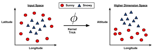
On the right side of the figure, after the kernel trick has been applied, we look at the data through the lens of a new dimension: Altitude. With the addition of this feature, the classes are now perfectly linearly separable. This is possible because we have obtained a new perspective on the data; in the left figure, we are viewing the mountain from a bird's-eye view, while on the right we are viewing the mountain from ground level. Here, the trend is obvious: snowy weather is found at higher altitudes.
SVMs with non-linear kernels add additional dimensions to the data in order to create separation in this way. Essentially, the kernel trick involves a process of adding new features that express mathematical relationships between measured characteristics. For instance, the altitude feature can be expressed mathematically as an interaction between latitude and longitude—the closer the point is to the center of each of these scales, the greater the altitude. This allows the SVM to learn concepts that were not explicitly measured in the original data.
SVMs with non-linear kernels are extremely powerful classifiers, although they do have some downsides as shown in the following table:
|
Strengths |
Weaknesses |
|---|---|
|
|
Kernel functions, in general, are of the following form. Here, the function denoted by the Greek letter phi, that is, ϕ(x), is a mapping of the data into another space:

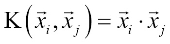
Using this form, kernel functions have been developed for many different domains of data. A few of the most commonly used kernel functions are listed as follows. Nearly all SVM software packages will include these kernels, among many others.
The linear kernel does not transform the data at all. Therefore, it can be expressed simply as the dot product of the features:
The polynomial kernel of degree d adds a simple non-linear transformation of the data:

The sigmoid kernel results in a SVM model somewhat analogous to a neural network using a sigmoid activation function. The Greek letters kappa and delta are used as kernel parameters:

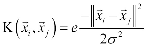
The Gaussian RBF kernel is similar to a RBF neural network. The RBF kernel performs well on many types of data and is thought to be a reasonable starting point for many learning tasks:
There is no reliable rule for matching a kernel to a particular learning task. The fit depends heavily on the concept to be learned as well as the amount of training data and the relationships among the features. Often, a bit of trial and error is required by training and evaluating several SVMs on a validation dataset. That said, in many cases, the choice of kernel is arbitrary, as the performance may vary only slightly. To see how this works in practice, let's apply our understanding of SVM classification to a real-world problem.