If you recall from Chapter 5, Divide and Conquer – Classification Using Decision Trees and Rules, a decision tree builds a model much like a flowchart in which decision nodes, leaf nodes, and branches define a series of decisions that can be used to classify examples. Such trees can also be used for numeric prediction by making only small adjustments to the tree growing algorithm. In this section, we will consider only the ways in which trees for numeric prediction differ from trees used for classification.
Trees for numeric prediction fall into two categories. The first, known as regression trees, were introduced in the 1980s as part of the seminal Classification and Regression Tree (CART) algorithm. Despite the name, regression trees do not use linear regression methods as described earlier in this chapter; rather, they make predictions based on the average value of examples that reach a leaf.
The second type of trees for numeric prediction is known as model trees. Introduced several years later than regression trees, they are less widely-known but perhaps more powerful. Model trees are grown in much the same way as regression trees, but at each leaf, a multiple linear regression model is built from the examples reaching that node. Depending on the number of leaf nodes, a model tree may build tens or even hundreds of such models. This may make model trees more difficult to understand than the equivalent regression tree, with the benefit that they may result in a more accurate model.
Trees that can perform numeric prediction offer a compelling yet often overlooked alternative to regression modeling. The strengths and weaknesses of regression trees and model trees relative to the more common regression methods are listed in the following table:
Though traditional regression methods are typically the first choice for numeric prediction tasks, in some cases, numeric decision trees offer distinct advantages. For instance, decision trees may be better suited for tasks with many features or many complex, non-linear relationships among features and the outcome; these situations present challenges for regression. Regression modeling also makes assumptions about how numeric data are distributed that are often violated in real-world data; this is not the case for trees.
Trees for numeric prediction are built in much the same way as they are for classification. Beginning at the root node, the data are partitioned using a divide-and-conquer strategy according to the feature that will result in the greatest increase in homogeneity in the outcome after a split is performed. In classification trees, you will recall that homogeneity is measured by entropy, which is undefined for numeric data. For numeric decision trees, homogeneity can be measured by statistics such as variance, standard deviation, or absolute deviation from the mean. Depending on the tree growing algorithm used, the homogeneity measure may vary, but the principles are basically the same.
A common splitting criterion is called the standard deviation reduction (SDR). It is defined by the following formula:
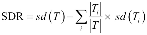
In this formula, the sd(T) function refers to the standard deviation of the values in set T, while T1 , T2 , … Tn are sets of values resulting from a split on a feature. The |T| term refers to the number of observations in set T. Essentially, the formula measures the reduction in standard deviation from the original value to the weighted standard deviation post-split.
For example, consider the following case, in which a tree is deciding whether to perform a split on binary feature A or a split on binary feature B:

Using the groups that would result from the proposed splits, we can compute the SDR for A and B as follows. The length() function used here returns the number of elements in a vector. Note that the overall group T is named tee to avoid overwriting R's built in T() and t() functions.
> tee <- c(1, 1, 1, 2, 2, 3, 4, 5, 5, 6, 6, 7, 7, 7, 7)
> at1 <- c(1, 1, 1, 2, 2, 3, 4, 5, 5)
> at2 <- c(6, 6, 7, 7, 7, 7)
> bt1 <- c(1, 1, 1, 2, 2, 3, 4)
> bt2 <- c(5, 5, 6, 6, 7, 7, 7, 7)
> sdr_a <- sd(tee) - (length(at1) / length(tee) * sd(at1) +
             length(at2) / length(tee) * sd(at2))
> sdr_b <- sd(tee) - (length(bt1) / length(tee) * sd(bt1) +
             length(bt2) / length(tee) * sd(bt2))
Let's compare the SDR of A against the SDR of B:
> sdr_a
[1] 1.202815
> sdr_b
[1] 1.392751
The SDR for the split on A was about 1.2 versus 1.4 for the split on B. Since the standard deviation was reduced more for B, the decision tree would use B first. It results in slightly more homogeneous sets than does A.
Suppose that the tree stopped growing here using this one and only split. The regression tree's work is done. It can make predictions for new examples depending on whether they fall into group T1 or T2. If the example ends up in T1, the model would predict mean(bt1) = 2, otherwise it would predict mean(bt2) = 6.25.
In contrast, the model tree would go one step further. Using the seven training examples falling in group bt1 and the eight in bt2, the model tree could build a linear regression model of the outcome versus feature A. (Feature B is of no help in the regression model because all examples at the leaf have the same value of B.) The model tree can then make predictions for new examples using either of the two linear models.
To further illustrate the differences between these two approaches, let's work through a real-world example.