To make a difficult decision, some people weigh their options by making lists of pros and cons for each possibility. Suppose a job seeker was deciding between several offers, some closer or further from home, with various levels of pay and benefits. He or she might create a list with the features of each position. Based on these features, rules can be created to eliminate some options. For instance, "if I have a commute longer than an hour, then I will be unhappy", or "if I make less than $50k, I won't be able to support my family." The difficult decision of predicting future happiness can be reduced to a series of small, but increasingly specific choices.
This chapter covers decision trees and rule learners—two machine learning methods that apply a similar strategy of dividing data into smaller and smaller portions to identify patterns that can be used for prediction. The knowledge is then presented in the form of logical structures that can be understood without any statistical knowledge. This aspect makes these models particularly useful for business strategy and process improvement.
By the end of this chapter, you will learn:
- The strategy each method employs to tackle the problem of partitioning data into interesting segments
- Several implementations of decision trees and classification rule learners, including the C5.0, 1R, and RIPPER algorithms
- How to use these algorithms for performing real-world classification tasks such as identifying risky bank loans and poisonous mushrooms
We will begin by examining decision trees and follow with a look at classification rules. Lastly, we'll wrap up with a summary of what we learned and preview later chapters, which discuss methods that use trees and rules as a foundation for other advanced machine learning techniques.
As you might intuit from the name, decision tree learners build a model in the form of a tree structure. The model itself comprises a series of logical decisions, similar to a flowchart, with decision nodes that indicate a decision to be made on an attribute. These split into branches that indicate the decision's choices. The tree is terminated by leaf nodes (also known as terminal nodes) that denote the result of following a combination of decisions.
Data that is to be classified begin at the root node where it is passed through the various decisions in the tree according to the values of its features. The path that the data takes funnels each record into a leaf node, which assigns it a predicted class.
As the decision tree is essentially a flowchart, it is particularly appropriate for applications in which the classification mechanism needs to be transparent for legal reasons or the results need to be shared in order to facilitate decision making. Some potential uses include:
- Credit scoring models in which the criteria that causes an applicant to be rejected need to be well-specified
- Marketing studies of customer churn or customer satisfaction that will be shared with management or advertising agencies
- Diagnosis of medical conditions based on laboratory measurements, symptoms, or rate of disease progression
Although the previous applications illustrate the value of trees for informing decision processes, that is not to suggest that their utility ends there. In fact, decision trees are perhaps the single most widely used machine learning technique, and can be applied for modeling almost any type of data—often with unparalleled performance.
In spite of their wide applicability, it is worth noting some scenarios where trees may not be an ideal fit. One such case might be a task where the data has a large number of nominal features with many levels or if the data has a large number of numeric features. These cases may result in a very large number of decisions and an overly complex tree.
Decision trees are built using a heuristic called recursive partitioning. This approach is generally known as divide and conquer because it uses the feature values to split the data into smaller and smaller subsets of similar classes.
Beginning at the root node, which represents the entire dataset, the algorithm chooses a feature that is the most predictive of the target class. The examples are then partitioned into groups of distinct values of this feature; this decision forms the first set of tree branches. The algorithm continues to divide-and-conquer the nodes, choosing the best candidate feature each time until a stopping criterion is reached. This might occur at a node if:
- All (or nearly all) of the examples at the node have the same class
- There are no remaining features to distinguish among examples
- The tree has grown to a predefined size limit
To illustrate the tree building process, let's consider a simple example. Imagine that you are working for a Hollywood film studio, and your desk is piled high with screenplays. Rather than read each one cover-to-cover, you decide to develop a decision tree algorithm to predict whether a potential movie would fall into one of three categories: mainstream hit, critic's choice, or box office bust.
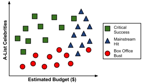
To gather data for your model, you turn to the studio archives to examine the previous ten years of movie releases. After reviewing the data for 30 different movie scripts, a pattern emerges. There seems to be a relationship between the film's proposed shooting budget, the number of A-list celebrities lined up for starring roles, and the categories of success. A scatter plot of this data might look something like the following diagram:
To build a simple decision tree using this data, we can apply a divide-and-conquer strategy. Let's first split the feature indicating the number of celebrities, partitioning the movies into groups with and without a low number of A-list stars:

Next, among the group of movies with a larger number of celebrities, we can make another split between movies with and without a high budget:

At this point we have partitioned the data into three groups. The group at the top-left corner of the diagram is composed entirely of critically-acclaimed films. This group is distinguished by a high number of celebrities and a relatively low budget. At the top-right corner, the majority of movies are box office hits, with high budgets and a large number of celebrities. The final group, which has little star power but budgets ranging from small to large, contains the flops.
If we wanted, we could continue to divide the data by splitting it based on increasingly specific ranges of budget and celebrity counts until each of the incorrectly classified values resides in its own, perhaps tiny partition. Since the data can continue to be split until there are no distinguishing features within a partition, a decision tree can be prone to be overfitting for the training data with overly-specific decisions. We'll avoid this by stopping the algorithm here since more than 80 percent of the examples in each group are from a single class.
Tip
You might have noticed that diagonal lines could have split the data even more cleanly. This is one limitation of the decision tree's knowledge representation, which uses axis-parallel splits. The fact that each split considers one feature at a time prevents the decision tree from forming more complex decisions such as "if the number of celebrities is greater than the estimated budget, then it will be a critical success".
Our model for predicting the future success of movies can be represented in a simple tree as shown in the following diagram. To evaluate a script, follow the branches through each decision until its success or failure has been predicted. In no time, you will be able to classify the backlog of scripts and get back to more important work such as writing an awards acceptance speech.

Since real-world data contains more than two features, decision trees quickly become far more complex than this, with many more nodes, branches, and leaves. In the next section you will learn about a popular algorithm for building decision tree models automatically.
There are numerous implementations of decision trees, but one of the most well-known is the C5.0 algorithm. This algorithm was developed by computer scientist J. Ross Quinlan as an improved version of his prior algorithm, C4.5, which itself is an improvement over his ID3 (Iterative Dichotomiser 3) algorithm. Although Quinlan markets C5.0 to commercial clients (see http://www.rulequest.com/ for details), the source code for a single-threaded version of the algorithm was made publically available, and has therefore been incorporated into programs such as R.
Note
To further confuse matters, a popular Java-based open-source alternative to C4.5, titled J48, is included in the RWeka package. Because the differences among C5.0, C4.5, and J48 are minor, the principles in this chapter will apply to any of these three methods and the algorithms should be considered synonymous.
The C5.0 algorithm has become the industry standard for producing decision trees, because it does well for most types of problems directly out of the box. Compared to other advanced machine learning models (such as those described in Chapter 7, Black Box Methods – Neural Networks and Support Vector Machines) the decision trees built by C5.0 generally perform nearly as well but are much easier to understand and deploy. Additionally, as shown in the following table, the algorithm's weaknesses are relatively minor and can be largely avoided.
Earlier in this chapter, we followed a simple example illustrating how a decision tree models data using a divide-and-conquer strategy. Let's explore this in more detail to examine how this heuristic works in practice.
The first challenge that a decision tree will face is to identify which feature to split upon. In the previous example, we looked for feature values that split the data in such a way that partitions contained examples primarily of a single class. If the segments of data contain only a single class, they are considered pure. There are many different measurements of purity for identifying splitting criteria.
C5.0 uses entropy for measuring purity. The entropy of a sample of data indicates how mixed the class values are; the minimum value of 0 indicates that the sample is completely homogenous, while 1 indicates the maximum amount of disorder. The definition of entropy is specified by:
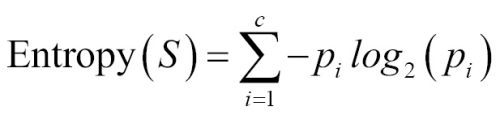
In the entropy formula, for a given segment of data (S), the term c refers to the number of different class levels, and pi refers to the proportion of values falling into class level i. For example, suppose we have a partition of data with two classes: red (60 percent), and white (40 percent). We can calculate the entropy as:
> -0.60 * log2(0.60) - 0.40 * log2(0.40)
[1] 0.9709506
We can examine the entropy for all possible two-class arrangements. If we know the proportion of examples in one class is x, then the proportion in the other class is 1 - x. Using the curve() function, we can then plot the entropy for all possible values of x:
> curve(-x * log2(x) - (1 - x) * log2(1 - x),
        col="red", xlab = "x", ylab = "Entropy", lwd=4)
This results in the following figure:

As illustrated by the peak in entropy at x = 0.50, a 50-50 split results in the maximum entropy. As one class increasingly dominates the other, the entropy reduces to zero.
Given this measure of purity, the algorithm must still decide which feature to split upon. For this, the algorithm uses entropy to calculate the change in homogeneity resulting from a split on each possible feature. The calculation is known as information gain. The information gain for a feature F is calculated as the difference between the entropy in the segment before the split (S1), and the partitions resulting from the split (S2):
The one complication is that after a split, the data is divided into more than one partition. Therefore, the function to calculate Entropy(S2 ) needs to consider the total entropy across all of the partitions. It does this by weighing each partition's entropy by the proportion of records falling into that partition. This can be stated in a formula as:

In simple terms, the total entropy resulting from a split is the sum of entropy of each of the n partitions weighted by the proportion of examples falling in that partition (wi).
The higher the information gain, the better a feature is at creating homogeneous groups after a split on that feature. If the information gain is zero, there is no reduction in entropy for splitting on this feature. On the other hand, the maximum information gain is equal to the entropy prior to the split. This would imply the entropy after the split is zero, which means that the decision results in completely homogeneous groups.
The previous formulae assume nominal features, but decision trees use information gain for splitting on numeric features as well. A common practice is testing various splits that divide the values into groups greater than or less than a threshold. This reduces the numeric feature into a two-level categorical feature and information gain can be calculated easily. The numeric threshold yielding the largest information gain is chosen for the split.
Note
Though it is used by C5.0, information gain is not the only splitting criterion that can be used to build decision trees. Other commonly used criteria are Gini index, Chi-Squared statistic, and gain ratio. For a review of these (and many more) criteria, refer to: An Empirical Comparison of Selection Measures for Decision-Tree Induction, Machine Learning, Vol. 3, pp. 319-342, by J. Mingers (1989).
A decision tree can continue to grow indefinitely, choosing splitting features and dividing into smaller and smaller partitions until each example is perfectly classified or the algorithm runs out of features to split on. However, if the tree grows overly large, many of the decisions it makes will be overly specific and the model will have been overfitted to the training data. The process of pruning a decision tree involves reducing its size such that it generalizes better to unseen data.
One solution to this problem is to stop the tree from growing once it reaches a certain number of decisions or if the decision nodes contain only a small number of examples. This is called early stopping or pre-pruning the decision tree. As the tree avoids doing needless work, this is an appealing strategy. However, one downside is that there is no way to know whether the tree will miss subtle, but important patterns that it would have learned had it grown to a larger size.
An alternative, called post-pruning involves growing a tree that is too large, then using pruning criteria based on the error rates at the nodes to reduce the size of the tree to a more appropriate level. This is often a more effective approach than pre-pruning because it is quite difficult to determine the optimal depth of a decision tree without growing it first. Pruning the tree later on allows the algorithm to be certain that all important data structures were discovered.
Note
The implementation details of pruning operations are very technical and beyond the scope of this book. For a comparison of some of the available methods, see: A comparative analysis of methods for pruning decision trees. IEEE Transactions on Pattern Analysis and Machine Intelligence, Vol. 19, pp. 476-491, by F. Esposito, D. Malerba, and G. Semeraro (1997).
One of the benefits of the C5.0 algorithm is that it is opinionated about pruning—it takes care of many of the decisions, automatically using fairly reasonable defaults. Its overall strategy is to postprune the tree. It first grows a large tree that overfits the training data. Later, nodes and branches that have little effect on the classification errors are removed. In some cases, entire branches are moved further up the tree or replaced by simpler decisions. These processes of grafting branches are known as subtree raising and subtree replacement, respectively.
Balancing overfitting and underfitting a decision tree is a bit of an art, but if model accuracy is vital it may be worth investing some time with various pruning options to see if it improves performance on the test data. As you will soon see, one of the strengths of the C5.0 algorithm is that it is very easy to adjust the training options.