On January 28, 1986, seven crewmembers of the United States space shuttle Challenger were killed when O-rings responsible for sealing the joints of the rocket booster failed and caused a catastrophic explosion.

The night prior, there had been a lengthy discussion about how the low temperature forecast might affect the safety of the launch. The shuttle components had never been tested in such cold weather; therefore, it was unclear whether the equipment could withstand the strain from freezing temperatures. The rocket engineers believed that cold temperatures could make the components more brittle and less able to seal properly, which would result in a higher chance of a dangerous fuel leak. However, given the political pressure to continue with the launch, they needed data to support their hypothesis.

The scientists' discussion turned to data from 23 previous successful shuttle launches which recorded the number of O-ring failures versus the launch temperature. Since the shuttle has a total of six O-rings, each additional failure increases the odds of a catastrophic leak. The following scatterplot shows this data:

Examining the plot, there is an apparent trend between temperature and number of failures. Launches occurring at higher temperatures tend to have fewer O-ring failures. Additionally, the coldest launch (62 degrees F) had two rings fail, the most of any launch. The fact that the Challenger was scheduled to launch at a temperature about 30 degrees colder seems concerning. To put this risk in quantitative terms, we can turn to simple linear regression.

Simple linear regression defines the relationship between a dependent variable and a single independent predictor variable using a line denoted by an equation in the following form:

Don't be alarmed by the Greek characters; this equation can still be understood using the slope-intercept form described previously. The intercept, α (alpha), describes where the line crosses the y axis, while the slope, β (beta), describes the change in y given an increase of x. For the shuttle launch data, the slope would tell us the expected reduction in number of O-ring failures for each degree the launch temperature increases.

Suppose we know that the estimated regression parameters in the equation for the shuttle launch data are:

Hence, the full linear equation is y = 4.30 – 0.057x. Ignoring for a moment how these numbers were obtained, we can plot the line on the scatterplot:

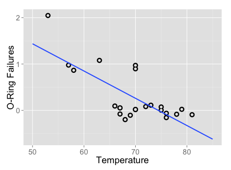
As the line shows, at 60 degrees Fahrenheit, we predict just under one O-ring failure. At 70 degrees Fahrenheit, we expect around 0.3 failures. If we extrapolate our model all the way out to 31 degrees—the forecasted temperature for the Challenger launch—we would expect about 4.30 – 0.057 * 31 = 2.53 O-ring failures. Assuming that each O-ring failure is equally likely to cause a catastrophic fuel leak, this means that the Challenger launch was about three times more risky than the typical launch at 60 degrees, and over eight times more risky than a launch at 70 degrees.

Notice that the line doesn't predict the data exactly. Instead, it cuts through the data somewhat evenly, with some predictions lower than expected and some higher. In the next section, we will learn about why this particular line was chosen.

In order to determine the optimal estimates of α and β, an estimation method known as ordinary least squares (OLS) was used. In OLS regression, the slope and intercept are chosen such that they minimize the sum of the squared errors, that is, the vertical distance between the predicted y value and the actual y value. These errors are known as residuals, and are illustrated for several points in the preceding diagram:

In mathematical terms, the goal of OLS regression can be expressed as the task of minimizing the following equation:

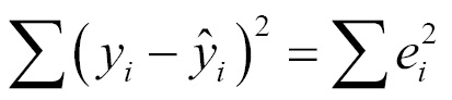
In plain language, this equation defines e (the error) as the difference between the actual y value and the predicted y value. The error values are squared and summed across all points in the data.

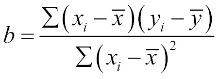
Though the proof is beyond the scope of this book, it can be shown using calculus that the value of b that results in the minimum squared error is:

While the optimal value of a is:

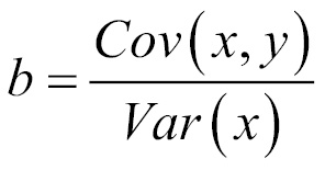
To understand these equations, we can break them into pieces. The denominator for b should look familiar; it is the same as the variance of x, which can be denoted as Var(x). As we learned in Chapter 2, Managing and Understanding Data, calculating the variance involves finding the average squared deviation from the mean of x.

We have not computed the numerator before. This involves taking the sum of each data point's deviation from the mean x value multiplied by that point's deviation away from the mean y value. This is known as the covariance of x and y, denoted as Cov(x, y). With this in mind, we can re-write the formula for b as:

Given this formula, it is easy to calculate the value of b using R functions. Assume that our shuttle launch data are stored in a data frame named launch, the independent variable x is temperature, and the dependent variable y is distress_ct. We can then use R's built-in cov() and var() functions to estimate b:

> b <- cov(launch$temperature, launch$distress_ct) /
         var(launch$temperature)
> b
[1] -0.05746032

From here, we can estimate a using the mean() function:

> a <- mean(launch$distress_ct) - b * mean(launch$temperature)
> a
[1] 4.301587

Estimating the regression equation in this way is not ideal, so R of course provides functions for doing this automatically. We will look at those shortly. First, we will expand our understanding of regression by learning a method for measuring the strength of a linear relationship and then see how linear regression can be applied to data having more than one independent variable.

The correlation between two variables is a number that indicates how closely their relationship follows a straight line. Without additional qualification, correlation refers to Pearson's correlation coefficient, which was developed by the 20th century mathematician Karl Pearson. The correlation ranges between -1 and +1. The extreme values indicate a perfectly linear relationship, while a correlation close to zero indicates the absence of a linear relationship.

The following formula defines Pearson's correlation:

Using this formula, we can calculate the correlation between the launch temperature and the number of O-ring failures. Recall that the covariance function is cov() and the standard deviation function is sd(). We'll store the result in r, a letter that is commonly used to indicate the estimated correlation:

> r <- cov(launch$temperature, launch$distress_ct) /
         (sd(launch$temperature) * sd(launch$distress_ct))
> r
[1] -0.725671

Alternatively, we can use the built in correlation function, cor():

> cor(launch$temperature, launch$distress_ct)
[1] -0.725671

Since the correlation is about -0.73, this implies that there is a fairly strong negative linear association between the temperature and the number of distressed O-rings. The negative association implies that an increase in temperature is correlated with fewer distressed O-rings. To the NASA engineers studying the O-ring data, this might have been a very clear indicator that a low-temperature launch could be problematic.

There are various rules-of-thumb used to interpret correlations. One method assigns a weak correlation to values between 0.1 and 0.3, moderate for 0.3 to 0.5, and strong for values above 0.5 (these also apply to similar ranges of negative correlations). However, these thresholds may be too lax for some purposes. Often, the correlation must be interpreted in context. For data involving human beings, a correlation of 0.5 may be considered extremely high; for data generated by mechanical processes, a correlation of 0.5 may be weak.

Measuring the correlation between two variables gives us a way to quickly gauge relationships among independent variables and the dependent variable. This will be increasingly important as we start defining regression models with a larger number of predictors.

Most real-world analyses have more than one independent variable. Therefore, it is likely that you will be using multiple linear regression most of the time you use regression for a numeric prediction task. The strengths and weaknesses of multiple linear regression are shown in the following table:

We can understand multiple regression as an extension of simple linear regression. The goal in both cases is similar: find values of beta coefficients that minimize the prediction error of a linear equation. The key difference is that there are additional terms for the additional independent variables.

Multiple regression equations generally follow the form of the following equation. The dependent variable y is specified as the sum of an intercept term plus the product of the estimated β value and the x value for each of i features. An error term (denoted by the Greek letter epsilon) has been added here as a reminder that the predictions are not perfect. This is the residual term noted previously.

Let's consider for a moment the interpretation of the estimated regression parameters. You will note that in the preceding equation, a coefficient is estimated for each feature. This allows each feature to have a separate estimated effect on the value of y. In other words, y changes by the amount β_i for each unit increase in x_i. The intercept is then the expected value of y when the independent variables are all zero.

Since the intercept is really no different than any other regression parameter, it can also be denoted as β₀ (pronounced beta-naught) as shown in the following equation:

This can be re-expressed using a condensed formulation:

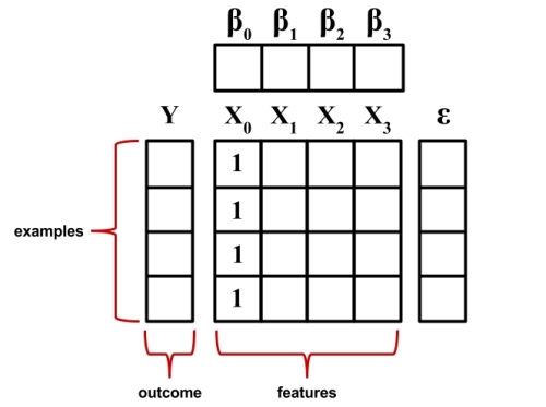
Even though this looks familiar, there are a few subtle changes. The dependent variable is now a vector, Y, with a row for every example. The independent variables have been combined into a matrix, X, with a column for each feature plus an additional column of '1' values for the intercept term. The regression coefficients β and errors ε are also now vectors.

The following figure illustrates these changes:

The goal now is to solve for the vector β that minimizes the sum of the squared errors between the predicted and actual y values. Finding the optimal solution requires the use of matrix algebra; therefore, the derivation deserves more careful attention than can be provided in this text. However, if you're willing to trust the work of others, the best estimate of the vector β can be computed as:

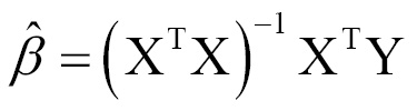
This solution uses a pair of matrix operations: the T indicates the transpose of matrix X, while the negative exponent indicates the matrix inverse. Using built-in R matrix operations, we can thus implement a simple multiple regression learner. Let's see if we can apply this formula to the Challenger launch data.

Using the following code, we can create a simple regression function named reg which takes a parameter y and a parameter x and returns a matrix of estimated beta coefficients.

> reg <- function(y, x) {
    x <- as.matrix(x)
    x <- cbind(Intercept = 1, x)
    solve(t(x) %*% x) %*% t(x) %*% y
  }

This function uses several R commands we have not used previously. First, since we will be using the function with sets of columns from a data frame, the as.matrix() function is used to coerce the data into matrix form. Next, the cbind() function is used to bind an additional column onto the x matrix; the command Intercept = 1 instructs R to name the new column Intercept and to fill the column with repeating 1 values. Finally, a number of matrix operations are performed on the x and y objects:

By combining these as shown in the formula for the estimated beta vector, our function will return estimated parameters for the linear model relating x to y.

Let's apply our reg() function to the shuttle launch data. As shown in the following code, the data include four features and the outcome of interest, distress_ct (the number of O-ring failures):

> str(launch)
'data.frame':	23 obs. of  5 variables:
 $ o_ring_ct  : int  6 6 6 6 6 6 6 6 6 6 ...
 $ distress_ct: int  0 1 0 0 0 0 0 0 1 1 ...
 $ temperature: int  66 70 69 68 67 72 73 70 57 63 ...
 $ pressure   : int  50 50 50 50 50 50 100 100 200 200 ...
 $ launch_id  : int  1 2 3 4 5 6 7 8 9 10 ...

We can confirm that our function is working correctly by comparing its result to the simple linear regression model of O-ring failures versus temperature, which we found earlier to have parameters a = 4.30 and b = -0.057. Since temperature is the third column of the launch data, we can run the reg() function as follows:

> reg(y = launch$distress_ct, x = launch[3])[,1]
Intercept    4.30158730
temperature -0.05746032

These values exactly match our prior result, so let's use the function to build a multiple regression model. We'll apply it just as before, but this time specifying three columns of data instead of just one:

> reg(y = launch$distress_ct, x = launch[3:5])[,1]
Intercept    3.814247216
temperature -0.055068768
pressure     0.003428843
launch_id   -0.016734090

This model predicts the number of O-ring failures versus temperature, pressure, and the launch ID number. The negative coefficients for the temperature and launch ID variables suggests that as temperature or the launch ID increases, the number of expected O-ring failures decreases. Applying the same interpretation to the coefficient for pressure, we learn that as the pressure increases, the number of O-ring failures is expected to increase.

So far, we've only scratched the surface of linear regression modeling. Although our work was useful to help understand exactly how regression models are built, R's functions for fitting linear regression models are not only likely faster than ours, but also more informative. Real-world regression packages provide a wealth of output to aid model interpretation. Let's apply our knowledge of regression to a more challenging learning task.